Article

Estimation of Paddy Rice Nitrogen Content and Accumulation Both at Leaf and Plant Levels from UAV Hyperspectral Imagery

1
Research Center of Guangdong Province for Engineering Technology Application of Remote Sensing Big Data, Key Lab of Guangdong for Utilization of Remote Sensing and Geographical Information System, Guangdong Open Laboratory of Geospatial Information Technology and Application, Guangzhou Institute of Geography, Guangdong Academy of Sciences, Guangzhou 510070, China
2
Institute of Agricultural Resources and Environment, Guangdong Academy of Agricultural Sciences, Guangzhou 510640, China
*
Author to whom correspondence should be addressed.
Remote Sens. 2021, 13(15), 2956; https://0-doi-org.brum.beds.ac.uk/10.3390/rs13152956
Submission received: 23 June 2021 / Revised: 20 July 2021 / Accepted: 22 July 2021 / Published: 27 July 2021
(This article belongs to the Special Issue Drones for Precision Agriculture: Remote Sensing Applications)

Abstract

:
Remote sensing-based mapping of crop nitrogen (N) status is beneficial for precision N management over large geographic regions. Both leaf/canopy level nitrogen content and accumulation are valuable for crop nutrient diagnosis. However, previous studies mainly focused on leaf nitrogen content (LNC) estimation. The effects of growth stages on the modeling accuracy have not been widely discussed. This study aimed to estimate different paddy rice N traits—LNC, plant nitrogen content (PNC), leaf nitrogen accumulation (LNA) and plant nitrogen accumulation (PNA)—from unmanned aerial vehicle (UAV)-based hyperspectral images. Additionally, the effects of the growth stage were evaluated. Univariate regression models on vegetation indices (VIs), the traditional multivariate calibration method, partial least squares regression (PLSR) and modern machine learning (ML) methods, including artificial neural network (ANN), random forest (RF), and support vector machine (SVM), were evaluated both over the whole growing season and in each single growth stage (including the tillering, jointing, booting and heading growth stages). The results indicate that the correlation between the four nitrogen traits and the other three biochemical traits—leaf chlorophyll content, canopy chlorophyll content and aboveground biomass—are affected by the growth stage. Within a single growth stage, the performance of selected VIs is relatively constant. For the full-growth-stage models, the performance of the VI-based models is more diverse. For the full-growth-stage models, the transformed chlorophyll absorption in the reflectance index/optimized soil-adjusted vegetation index (TCARI/OSAVI) performs best for LNC, PNC and PNA estimation, while the three band vegetation index (TBVITian) performs best for LNA estimation. There are no obvious patterns regarding which method performs the best of the PLSR, ANN, RF and SVM in either the growth-stage-specific or full-growth-stage models. For the growth-stage-specific models, a lower mean relative error (MRE) and higher R2 can be acquired at the tillering and jointing growth stages. The PLSR and ML methods yield obviously better estimation accuracy for the full-growth-stage models than the VI-based models. For the growth-stage-specific models, the performance of VI-based models seems optimal and cannot be obviously surpassed. These results suggest that building linear regression models on VIs for paddy rice nitrogen traits estimation is still a reasonable choice when only a single growth stage is involved. However, when multiple growth stages are involved or missing the phenology information, using PLSR or ML methods is a better option.

Graphical Abstract

1. Introduction

Nitrogen (N) is one of the most important plant macronutrients and plays a significant role in the photosynthesis process. It is important for crop development, production and quality [1,2,3]. Proper N fertilization can help crops achieve maximum potential yield [4]. However, the uncertainty in the climate of the current year, previous crop management, and soil N supply cause actual N uptake to vary in both time and space. N deficiency can negatively affect photosynthesis and biomass accumulation, as well as both the quality and quantity of the crop yield [5]. Thus, considering the relatively low cost of N fertilization, overapplication of N fertilizer is a common phenomenon in agricultural practice to ensure maximum yield [6]. The overapplication of N fertilizer can result in problems such as plant stress, the overproduction of leaves, and more unproductive tillers. Additionally, it increases the N leaching risk of cropping systems.
For early growth stages, monitoring the crop N content can help in fertilization planning. For maturing growth stages, monitoring crop N content can help indicate yield quality [7]. Thus, the continuous monitoring of crop N content is of great importance. The destructive determination of N content, using chemical methods such as the Kjeldahl technique, is laborious, lengthy and costly [5]. Portable chlorophyll meters, such as SPAD- 502, can be used to quickly diagnose crop N status. These tools are still point-sampling based and not suitable for precision N management across large areas. Remote sensing, however, provides a cost-effective and nondestructive avenue for monitoring crop N status over large geographic areas [8]. Using radiometric data to map crop N conditions has been reported for many crops.
Although there are a few works trying to use radiation transformation models, such as N-PROSPECT [9] or PROPSECT-PRO [10], which are modified versions of the widely used PROSPECT model [11], for N content estimation, remote sensing-based crop N content detection is mainly conducted using empirical relationships from vegetation indices (VIs) that are sensitive to chlorophyll content based on the fact that the two variables are moderately to be highly correlated [12]. Tian et al. [13] quantified the relationship between paddy rice leaf nitrogen content (LNC) and red-edge position (REP) with different algorithms. Li et al. [14] found that the canopy chlorophyll content index (CCCI) and N planar domain index (NDPI) are stable predictors for wheat plant nitrogen content (PNC) after the heading growth stage. Patel et al. [15] evaluated the relationships of several popular broadband VIs with the PNC, plant nitrogen accumulation (PNA) and aboveground biomass (ABG) of ryegrass. Li et al. [16] evaluated several hyperspectral VIs for winter wheat PNC estimation across different years and growth stages. Fitzgerald et al. [17] suggested that the CCCI is suitable for predicting rainfall wheat PNC at the stem elongation growth stage.
There are also studies trying to build VIs that are directly related to N traits. Lee et al. [18] suggested that the first derivative of canopy spectra at 735 nm is a good indicator for the PNC of paddy rice at the panicle formation stage. Stroppiana et al. [19] concluded that the normalized difference vegetation index (NDVI) formulated with narrow band reflectance at 483 nm and 503 nm was optimal for paddy rice PNC estimation in a combined data set from panicle initiation and heading stages. They also pointed out that VIs specially designed for chlorophyll/nitrogen estimation, such as the transformed chlorophyll absorption in reflectance index (TCARI) and modified chlorophyll absorption ratio index (MCARI) did not perform well in their data set. Tian et al. [20] proposed a three band index that performed well at both the ground and space scales for paddy rice LNC estimation.
Considering that VIs typically use two to three bands, univariate regression models built on VIs are criticized because they do not fully take advantage of spectrometric data (in particular, hyperspectral data) and may be too simple to characterize the intrinsic relationships between the target variable and spectrometric data [21,22,23,24]. Partial least squares regression (PLSR) is a powerful alternative method and can perform better for biochemical trait estimation in most cases [25,26,27,28,29,30]. Specifically, Hansen and Schjoerring [24] showed that PLSR could reduce the root mean square error (RMSE) of LNC estimation by 24%, compared to those of narrowband VIs. More recently, state-of-art machine learning (ML) methods, such as artificial neural networks (ANNs), random forests (RFs) and support vector machines (SVMs), were evaluated for N trait estimation and yielded encouraging results [31,32,33,34,35,36,37,38].
Most of the previous studies focused on special narrow growth stages, such as the early season [32], stem elongation stage [17], panicle initiation stage [18,26,39], heading stage [14], and anthesis stage [40]. Additionally, the LNC is usually considered the target variable [1]. However, the N content can be expressed both per dry weight and per unit surface. Additionally, the N content can be measured at the leaf scale and at the wholeplant scale. The growth stage development is accompanied by canopy structure variation, biomass accumulation and N allocation. How the prediction strength of spectrometric data for different N traits varies across growth stages has not been fully explored. Therefore, the objective of this study is to evaluate the performance of VIs, PLSR and ML methods for paddy rice N trait estimation, with a special focus on the effects of growth stages.

2. Materials and Methods

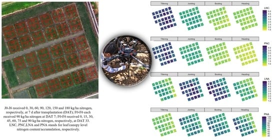
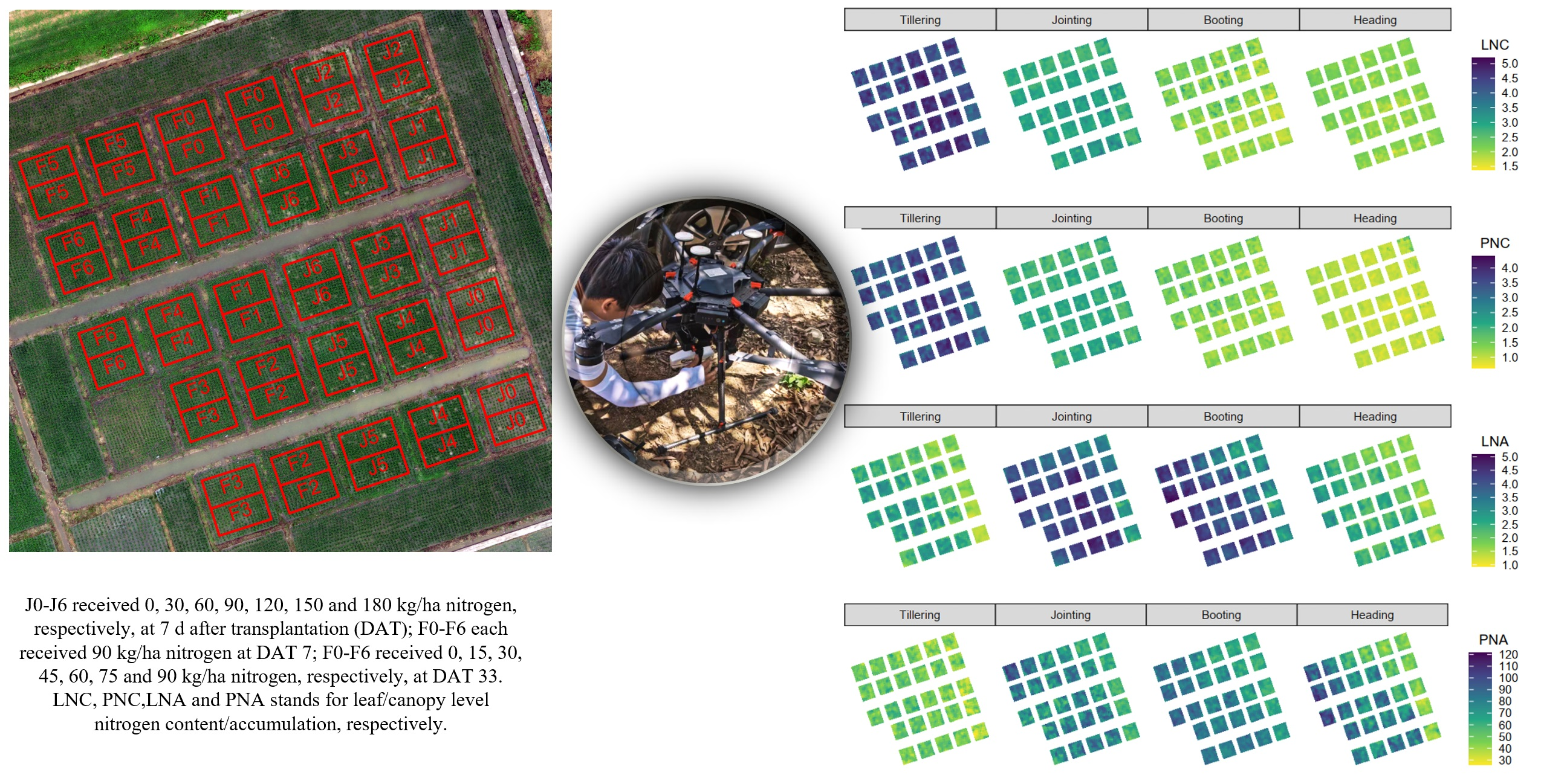
2.1. Study Area and Experimental Setup

The experiments were conducted at the rice research field of Guangdong Academy of Agricultural Sciences (23°23′38″N, 113°25′37″E). This region is characterized by a subtropical monsoon climate. The average annual precipitation and average temperature are 1700 (mm) and 22.5 °C, respectively. The parent material of the soil in the test area is lateritic sandy loam formed by river alluvium. In this region, paddy rice is under a two-season cropping system. Our experiments were conducted during the 2020 late rice growing season. The paddy rice variety Huangruanxiuzhan was used as the test material. The paddy rice was sown in a nursery bed and manually transplanted on 9 August 2020. The transplanting density was 400 plants/plot with one plant per hill.
To acquire the necessary reference observations, a paddy rice field with nitrogen treatment was set up and used to conduct field-data collection campaigns (detailed in Figure 1). Nitrogen from 0 to 180 (kg ha−1) with a 30 (kg ha−1) increase was applied to plots J0 to J6 7d after transplantation (DAT). Nitrogen from 0 to 90 (kg ha−1) with an  15 (kg ha−1) increase was applied to plots F0 to F6 at  33 DAT. Additionally, 90 (kg ha−1) nitrogen was applied to each plot from F0 to F6 at 7 DAT. The paddy rice was at the tillering and jointing growth stages at  7 and  33 DAT, respectively. Phosphates and potash fertilizers were applied as basal dressings with P2O5 and K2O at 45 and 120 (kg ha−1), respectively, for each plot. For both J0 to J6 and F0 to F6, each nitrogen level comprised two replicates. Thus, there were 28 plots in total. Each plot was (5 × 4.5 m) in size.

2.2. Field Data Collection
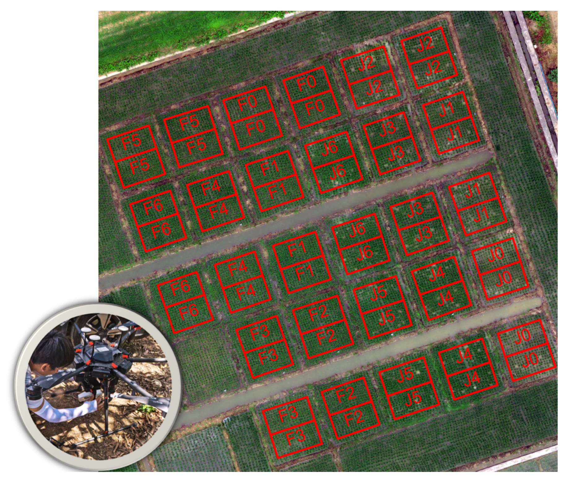
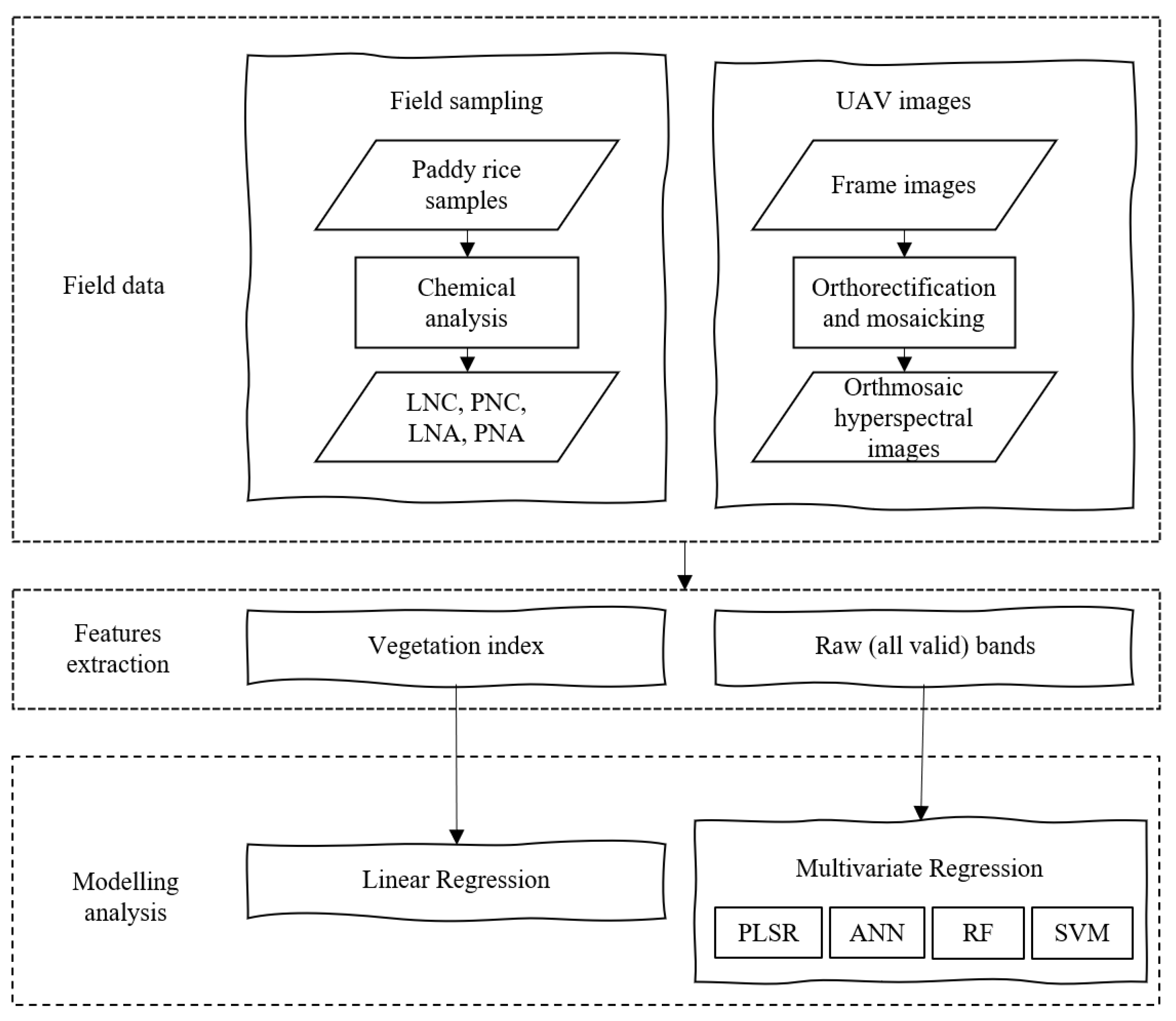
Four field-data collection campaigns were carried out at 18, 32, 47 and 62 DAT. The paddy rice was in the tillering, jointing, booting, and heading growth stages on the corresponding dates. The growth stage was determined, according to the rules described by [41].
Each plot was equally split into two sampling areas (demonstrated in Figure 1). For each field-data collection campaign, the grazeable biomass of three to five hill plants of each sampling area was randomly destructively sampled. Then, the sample plants were split into two parts: green leaves and other (senescent leaves, stems and particles). For each sample, 30 random SPAD-502 (Minolta Camera Co., Osaka, Japan) readings were recorded on green leaves. Then, all green leaves were scanned by a portable scanner (PERFECTION V39, Seiko Epson Corp., Nagano, Japan). The soil plant analysis development (SPAD) readings were converted to leaf chlorophyll content (LCC) (mg cm−2) with an empirical relationship (Equation (1)) proposed by [42] and averaged as the LCC of the corresponding sampling area. The leaf pixels in scanned images were extracted by a threshold method. The leaf area indices (LAIs) of each sampling area were determined by Equation (2), where ρ g r e e n l e a f is the green-leaf pixel ratio of each scanned image, a r e a i m g = 216 × 297 × 10 4 m is the maximum scan area of the scanner, and d e n s i t y = 400 / ( 5 × 4.5 ) m 2 is the planting density. The canopy chlorophyll content (CCC) was approximated by multiplying the LAI and LCC (Equation (3)).
LCC = 99 × S P A D / ( 144 S P A D )
LAI = 1 d e n s i t y ( ρ g r e e n l e a f × a r e a i m g )
CCC = LAI × LCC
In the second step, samples were oven-dried at 105 °C for half an hour and then at 75 °C until a constant weight was reached. Finally, the oven-dried samples of different organs were weighed and used to determine the leaf biomass, ABG, nitrogen content (Kjeldahl method) and accumulation. Both LNC and PNC were measured. Additionally, LNA and PNA were determined by multiplying LNC and PNC with leaf biomass and ABG, respectively.
Plots J0 to J6 were sampled during data collection campaigns at 18, 32 and 47 DAT, while plots F0 to F6 were sampled during data collection campaigns at 47 and 62 DAT. Thus, 28 samples were acquired for each data collection campaign, except for 47 DAT (56 samples).
Canopy reflectance data were acquired by a Cubert S185 hyperspectral camera (Cubert GmbH, Ulm, Germany) installed on a hexacopter (DJI M600Pro, SZ DJI Technology Co., Shenzhen, Guangzhou, China). The hyperspectral camera has a spectral range of 450–950 nm and a spectral resolution of 4 nm. It was installed through a three-axis gimbal stabilizer (DJI Ronin-MX, SZ DJI Technology Co., Shenzhen, Guangzhou, China). All unmanned aerial vehicle (UAV) flight missions were performed at approximately 11:00 a.m. Considering that the camera viewing angle may affect the estimation of the canopy parameters [43,44], the same view angle was ensured by the gimbal stabilizer to acquire the nadir images. The flight height was 30 m, which resulted in 16 cm spatial resolution for hyperspectral images. The hyperspectral images were mosaicked and orthographically projected for further analysis. The bands beyond 850 nm were dropped because of the low spectral quality [45]. The sample-area-wise mean spectra were calculated using regions of interest generated from sample area boundaries (demonstrated in Figure 1).

2.3. Methods

Linear regression models based on VIs, as well as PLSR and three ML models (ANN, RF and SVM) based on raw reflectance spectra, were built. Both full-growth-stage and growth-stage-specific models were built for each nitrogen trait (LNC, PNC, LNA and PNA). The general workflow is demonstrated in Figure 2. All models were built in the R environment [46]. The PLSR, ANN, RF and SVM models were built using the R packages plsmod [47], nnet [48], randomForest [49] and kernlab [50], respectively.
Twenty-three VIs were evaluated in this study (listed in Table 1). These indices are commonly used for biomass, chlorophyll and nitrogen status estimation. Specifically, the CCCI [17] is a two-dimensional index based on the normalized difference red edge (NDRE) and NDVI. By capturing the planar domain idea proposed by Clarke et al. [51], the CCCI attempts to separate the soil background signal from the plant signal. The NDVI is used as a surrogate for ground cover, and the NDRE is used as a measure of nitrogen content. Conceptually, this allows the nitrogen for any ground cover to be measured. Similarly, Li et al. [14] proposed the NDPI by changing the NDRE in CCCI to CIre.
A detailed description of the PLSR, ANN, RF and SVM methods can be found in our previous work [21]. In this work, a single-hidden-layer neural network structure was used for the ANN; a radial basis kernel function (RBF) was used for the SVM. In these methods, the latent variables (LVs) of the PLSR, the number of hidden units (units) of the ANN, the number of randomly selected variables of each tree (mtry) and the number of trees (ntree) of the RF, and the σ in the RBF and the C-constant of the regularization term in the Lagrange formulation of the SVM are hyperparameters that need to be fine tuned.
The full-growth-stage models were built on the full data set, while the growth-stage-specific models were built on the data of the corresponding growth stages. The corresponding data set was randomly split into calibration and validation data sets at a 3:1 ratio. All models were calibrated and validated on the calibration and validation data sets, respectively. The mean relative error (MRE), RMSE and coefficient of determination (R2) were calculated to evaluate the model performance (Equations (4)–(6)), where Oi and Pi are the ith observed and predicted data, respectively, and n is the size of the data pairs.
R 2 = 1 i = 1 n ( O i P i ) 2 i = 1 2 ( O i P i ) 2
RMSE = i = 1 n ( O i P i ) 2 n
MRE = 100 % 1 n i = 1 n | O i P i | O i
For the PLSR, ANN, RF and SVM, the hyperparameters (LVs for the PLSR, units for the ANN, mtry for the RF and C, σ for the SVM) were determined by a grid search with a repeated (5 times) 10-fold cross-validation procedure on the calibration data set (Algorithm 1). The parameter (or parameter combination) associated with the lowest MREcv was considered optimal. After the key parameters were determined, the final models were calibrated on the corresponding calibration data set and evaluated on the corresponding standalone validation data set. Although no hyperparameters needed to be determined for the linear models based on VIs, the same cross-validation procedure was used to calculate the cross-validated calibration MREcv, RMSEcv, R c v 2 . The same fold split scheme across different models (of the same growth stage) was used to ensure a fair comparison. MREcv, RMSEcv and R c v 2 were mainly used for model performance comparison.
Algorithm 1: Hyperparameter optimization and model calibration algorithm.
Remotesensing 13 02956 i001

3. Results

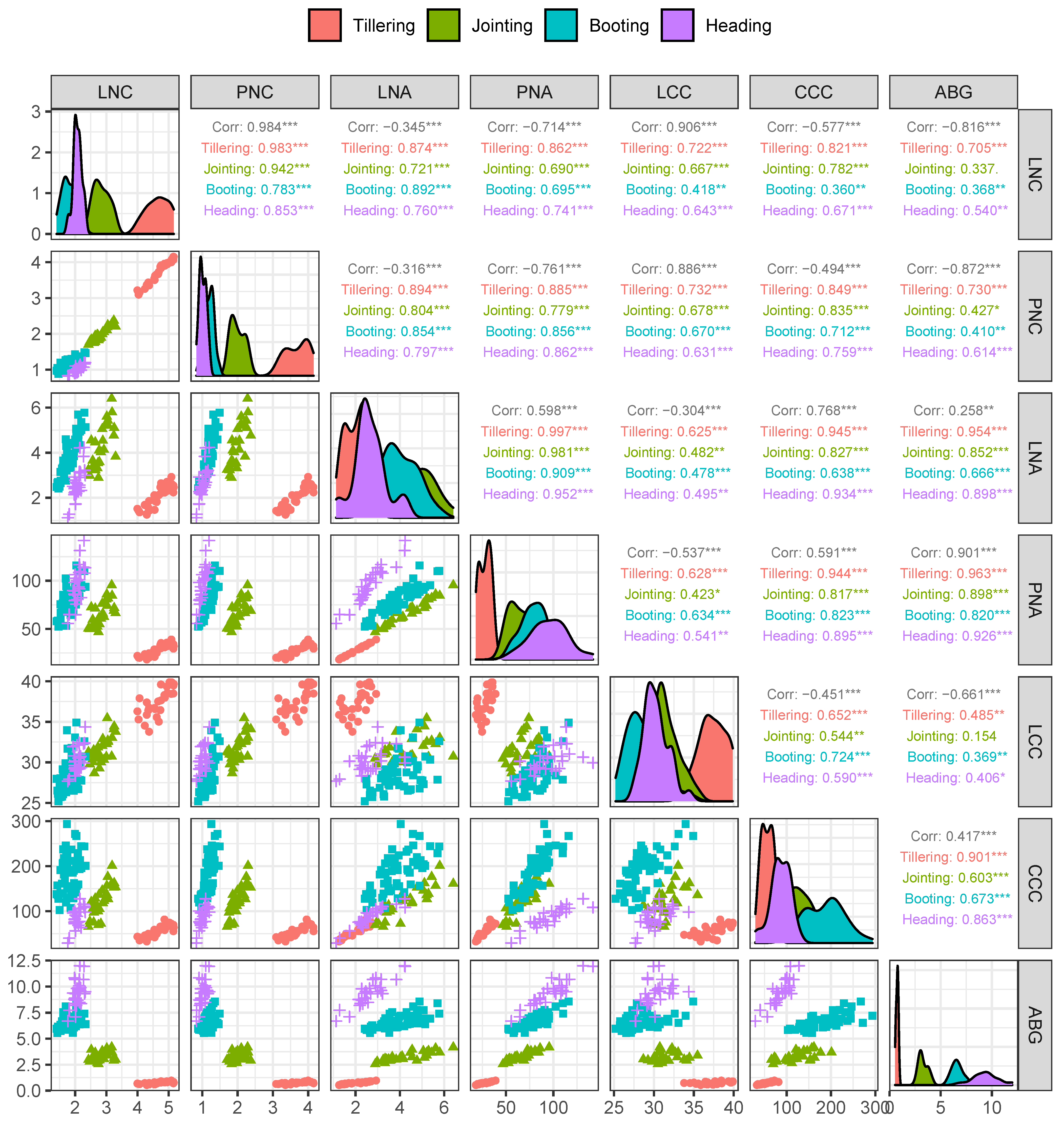
3.1. Variability in the Measured Nitrogen, Chlorophyll and Aboveground Biomass

Table 2 depicts the variation in the measured LNC, PNC, LNA, PNA, LCC, CCC and ABG. In the full data set (with all growth stages combined), the LNC varies from 1.41% to 5.16% with coefficient of variation (CV) at 38.63%, the PNC varies from 0.83% to 4.15% with CV at 56.29%, the LNA varies from 1.12 g m−2 to 6.41 g m−2 with CV at 33.04%, the PNA varies from 18.21 kg ha−1 to 156.36 kg ha−1 with CV at 39.85%, the LCC varies from 22.38 μg cm−2 to 39.88 μg cm−2 with CV at 12.44%, the CCC ranges from 29.39 μg cm−2 to 293.72 μg cm−2 with CV at 51.98%, and the ABG varies from 0.54 t ha−1 to 12.38 t ha−1 with CV at 54.24%.
The means of LNC and PNC generally show a decreasing pattern from the tilling to heading growth stages, due to dilution effects [4]. Apart from that, the mean LNC at the heading growth stage is slightly higher than the mean at the booting growth stage. This is because our LNC is measured on the green leaves. During the heading growth stage, nitrogen is allocated from senescent leaves to young (green) leaves, which yields a LNC higher than that measured by combining senescent and green leaves together. The means of LCC show a pattern similar to those of LNC. The means of LNA and CCC first increase and then decrease from the tillering to heading growth stages. The means of PNA and ABG show an increasing pattern from the tillering to heading growth stages. The CV of each trait is lower for the single growth stage (data collection campaign) than for the full data set. The maximum values of the ratio between the single growth stage CV and full data set CV are 0.34, 0.20, 0.83, and 0.55 for LNC, PNC, LNA, and PNA, respectively.
Figure 3 shows the pairwise scatter plots and correlation coefficients of all seven traits (LNC, PNC, LNA, PNA, LCC, CCC and ABG). LNC is more correlated with LCC than CCC and ABG regardless of whether for the full dataset or a specific growth stage. PNC is highly correlated with LNC regardless of whether it is for the full data set or a specific growth stage. However, PNC is more correlated with LCC than CCC and ABG on the full data set, similar to LNC. However, at a specific growth stage, PNC is more correlated with CCC. Both LNA and PNA are more correlated with ABG than LCC and CCC for almost all specific growth stages. For the full data set, LNA is more correlated with CCC, and PNA is more correlated with ABG of the LCC, CCC and ABG traits. Except for LNC vs. PNC, all other pairwise relationships between LNC, PNC, LNA, PNA, LCC, CCC and ABG are affected by the growth stages. Although the growth-stage-specific correlation coefficients are positive, the full data set correlation coefficients of LNC vs. CCC, LNC vs. ABG, PNC vs. CCC, PNC vs. ABG, LNA vs. LCC, and PNA vs. LCC are negative.

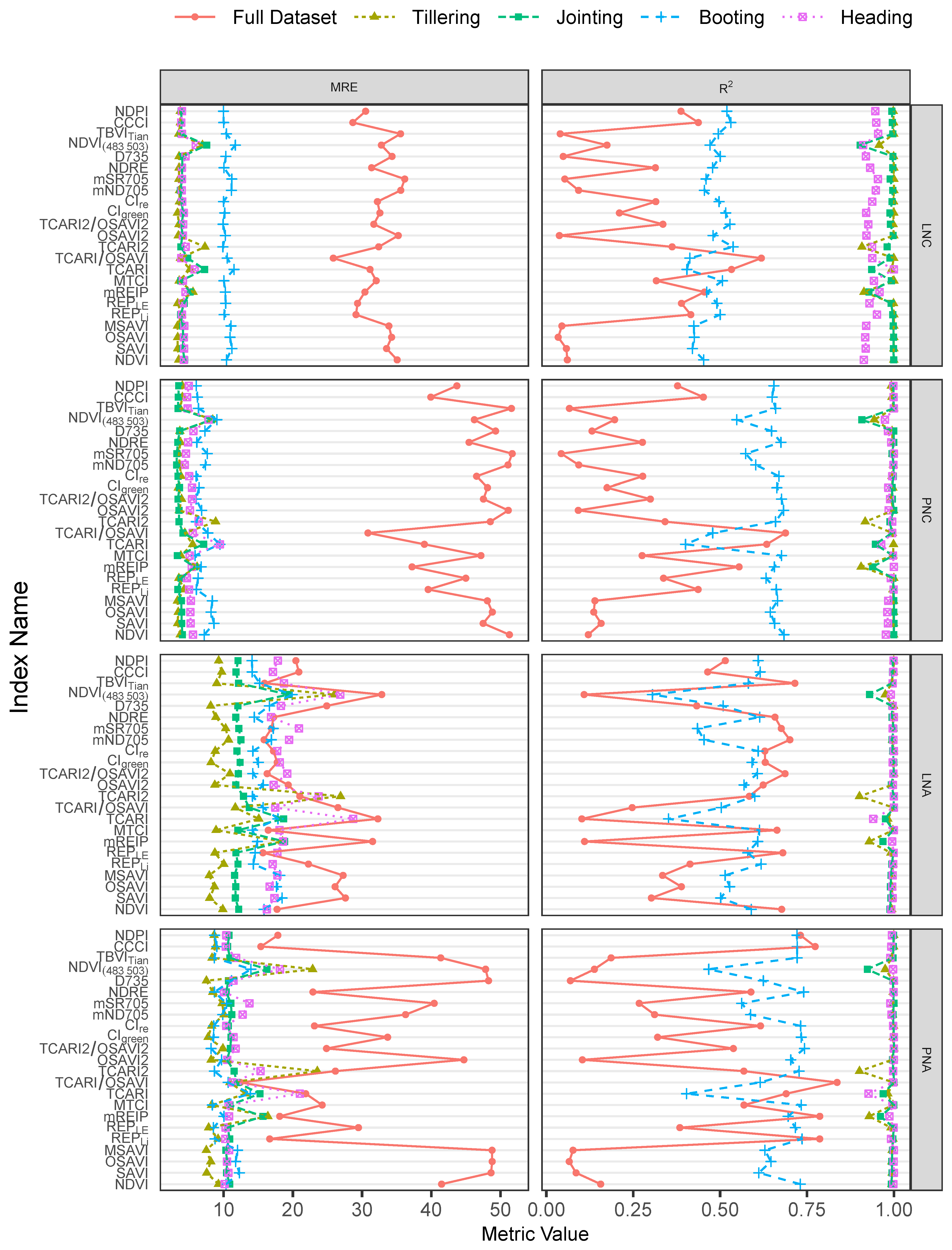
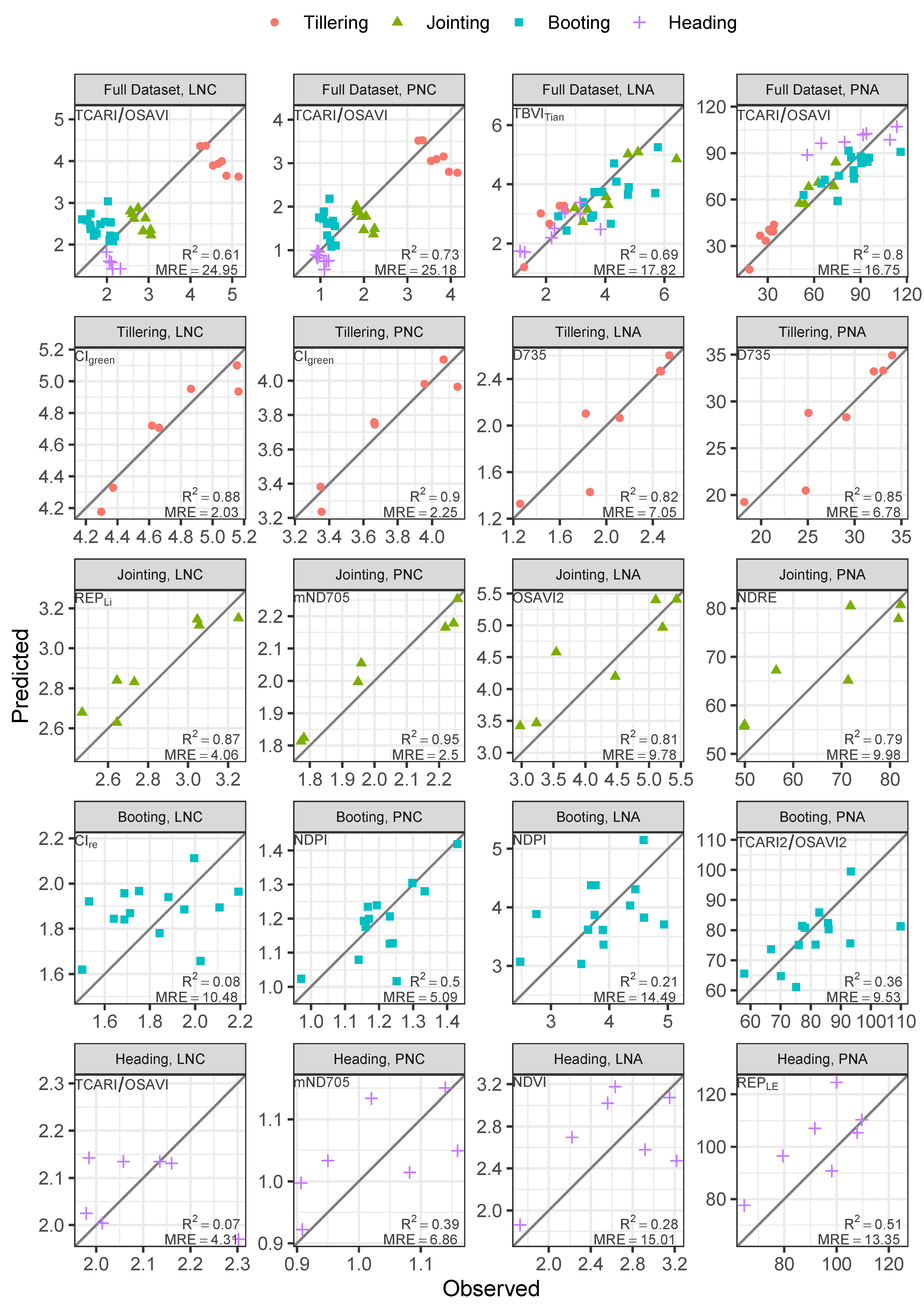
3.2. Performance of the VIs

Figure 4 depicts the full-growth-stage and growth-stage-specific MREcv and R c v 2 of selected VIs for LNC, PNC, LNA and PNA prediction. For growth-stage-specific models of each tillering, jointing and heading growth stage, almost all selected VIs show good performance with relatively low MREcv and high R c v 2 values for all four nitrogen traits, except for TCARI and NDVI483,503, whose performance is slightly worse than that of the other VIs. For the booting growth stage, the R c v 2 values of the growth-stage-specific models are lower than those of the other three growth stages for all four nitrogen traits. For the full-growth-stage models, the performance of all selected VIs is lower than the corresponding growth-stage-specific models (except for the booting growth stage).
The performance of the selected VIs is more diverse in the full-growth-stage models and booting growth stage growth-stage-specific models than in tillering, jointing and heading growth stage growth-stage-specific models. The MREcv values of the growth-stage-specific models for LNC and PNC are generally lower than those of the corresponding models for LNA and PNA. The MREcv values of the full-growth-stage models for LNA and PNA are generally lower than those of the corresponding models for LNC and PNC.
Table 3 lists the best-performing VI according to the MREcv values for each full-growth-stage and growth-stage-specific model of each nitrogen trait. Figure 5 shows the scatter plot between the observed and predicted nitrogen traits in the corresponding validation data set of these models. For full-growth-stage models, the transformed chlorophyll absorption in the reflectance index/optimized soil-adjusted vegetation index (TCARI/OSAVI) yields the lowest MREcv values for LNC and PNC and PNA, while the three band vegetation index (TBVITian) yields the lowest MREcv for LNA. The validation MRE (MREval) values are 24.95%, 25.18%, 17.82% and 16.75% and the validation R2 (R v a l 2 ) values are 0.61, 0.73, 0.69 and 0.80 for LNC, PNC, LNA and PNA, respectively. The full-growth-stage models of LNA and PNA could yield lower MRE and higher R2 values than LNC and PNC both in model calibration and validation.
For growth-stage-specific models, the MRE and R2 range from 3.34% to 10.48% and 0.08 to 1.00 for LNC in both model calibration and validation. According to MREcv, the model performances are ordered as follows: tillering > jointing > heading > booting. The MRE and R2 range from 3.20% to 6.86% and 0.39 to 1.00 for PNC in both model calibration and validation. The model performance order is similar to that of LNC. The validation MRE and R2 range from 7.05% to 16.24% and 0.21 to 1.00 for LNA in both model calibration and validation. According to MREcv, the model performances are ordered as follows: tillering > jointing > booting > heading. The MRE and R2 range from 6.78% to 13.35% for PNA in both model calibration and validation. According to MREcv, the model performances are ordered as follows: tillering > booting > heading > jointing. For each nitrogen trait, the growth-stage-specific model always yields a lower MRE in both model calibration and validation than the corresponding full-growth-stage models.

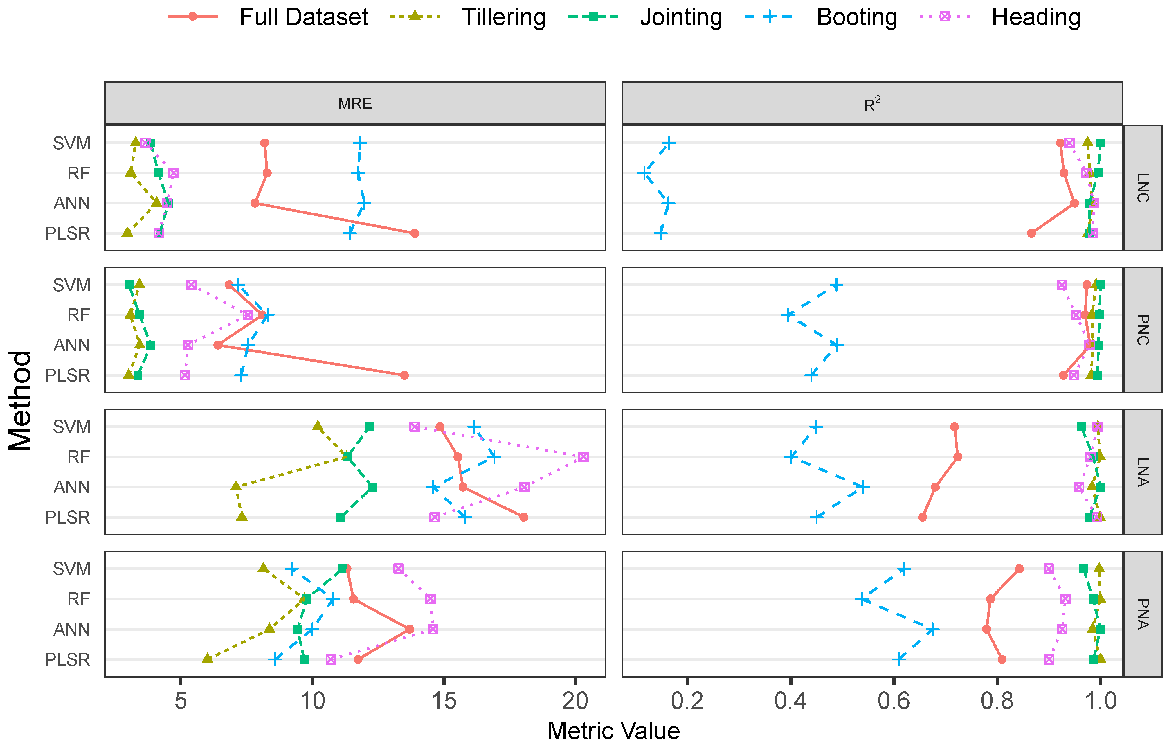
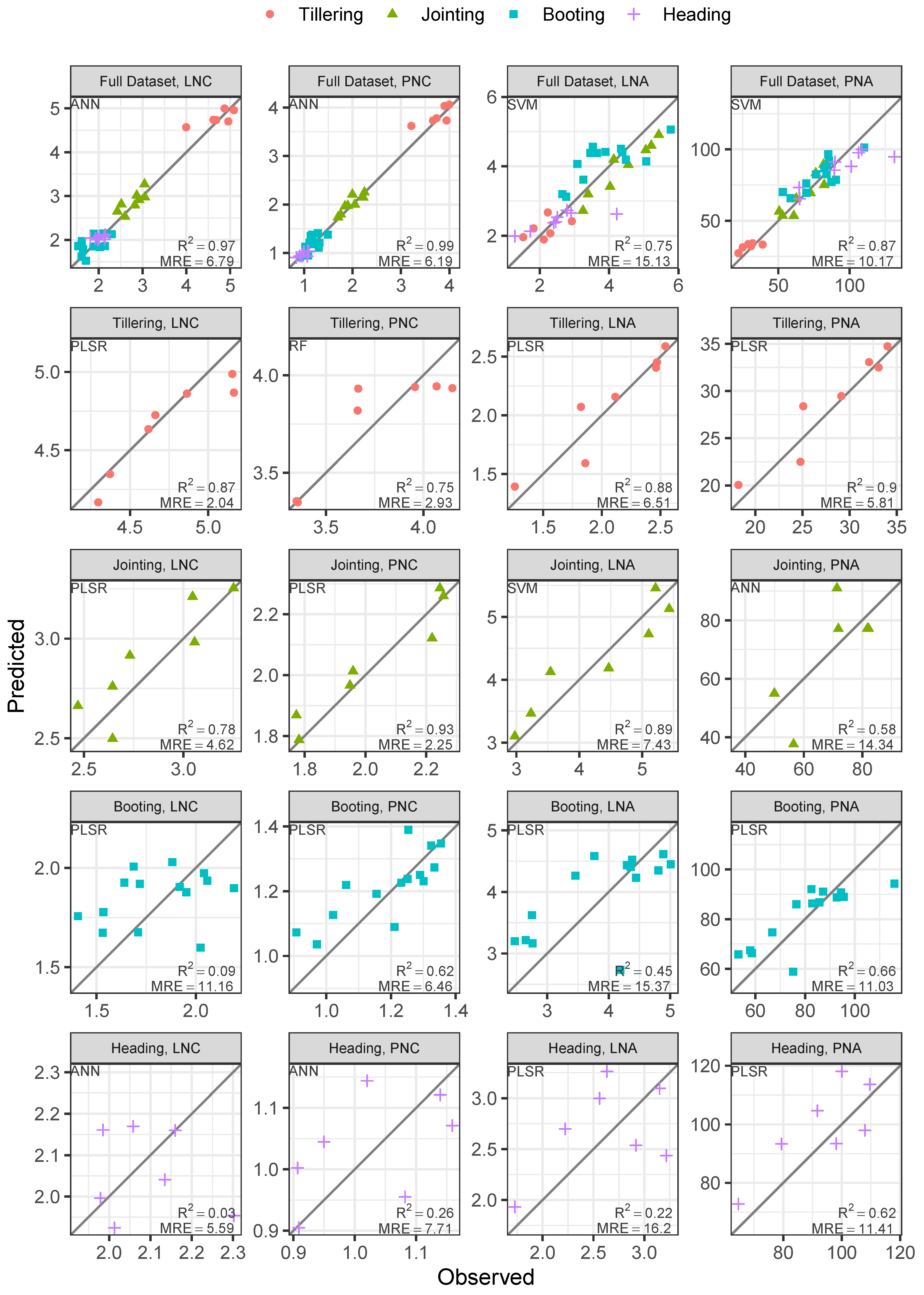
3.3. Performance of the PLSR and ML Methods

Figure 6 shows the growth-stage-specific and full-growth-stage MREcv and R c v 2 values of the PLSR and three ML methods (the ANN, RF and SVM) for the four nitrogen traits (LNC, PNC, LNA and PNA). There are no obvious patterns showing a certain method clearly outperforming the other methods. However, the PLSR may yield a large MREcv in the full-growth-stage models. Of the four nitrogen traits, the booting growth stage models yield the lowest Rcv and moderate or highest MREcv of the growth-stage-specific models and full-growth-stage models.
For LNC and PNC, the full-growth-stage models yield R c v 2 values comparable to those of the tillering, jointing and heading growth-stage-specific models. For LNA and PNA, the full-growth-stage models yield slightly lower R c v 2 values than the tillering, jointing and heading growth-stage-specific models. However, the R c v 2 values are still above 0.60. The MREcv values of LNC and PNC are slightly lower than the corresponding MRE values of LNA and PNA.
Table 4 lists the best-performing models of the full-growth-stage and each growth-stage-specific models for LNC, PNC, LNA and PNA selected by MREcv. Figure 7 shows the scatter plots between the observed and predicted nitrogen traits in the corresponding validation data sets. In the full-growth-stage models, the ANN method outperforms the other three methods for LNC and PNC, while the SVM outperforms the other three methods for LNA and PNA. For both LNC and PNC, the full-growth-stage models built on the ANN yield MRE below 7.82% and R2 above 0.95 both in model calibration and validation. For LNA and PNA, the performance of the full-growth-stage models slightly degrades. The MRE ranges between 11.04% and 14.85%, and R2 ranges between 0.72 and 0.87 in both model calibration and validation.
For LNC, only the tillering growth-stage-specific model yields good performance, with MRE below 3.38% and R2 above 0.86 in both model calibration and validation. Although the growth-stage-specific models of the other three growth stages (jointing, booting and heading) yield lower MREval, the R v a l 2 values are lower (ranging between 0.01 and 0.50). For LNA, all tillering, jointing and heading growth-stage-specific models yield good performance, with MRE below 28.26% and R2 above 0.84 in both model calibration and validation. The booting growth-stage-specific model yields lower R v a l 2 (R v a l 2 = 0.22). For both PNC and PNA, the growth-stage-specific models from tillering to heading growth stages all show good performance, with MRE below 10.83% and R2 above 0.44 in both model calibration and validation.
Comparing Table 3 and Table 4, which present the best-performing VI-based and full-spectra-based models, respectively, the latter is clearly superior, regarding the full-growth-stage models of each nitrogen trait. The VI-based growth-stage-specific model of the booting growth stage yields lower accuracy for each nitrogen trait. With the full-spectra-based models, the prediction accuracy is improved for PNC and PNA.

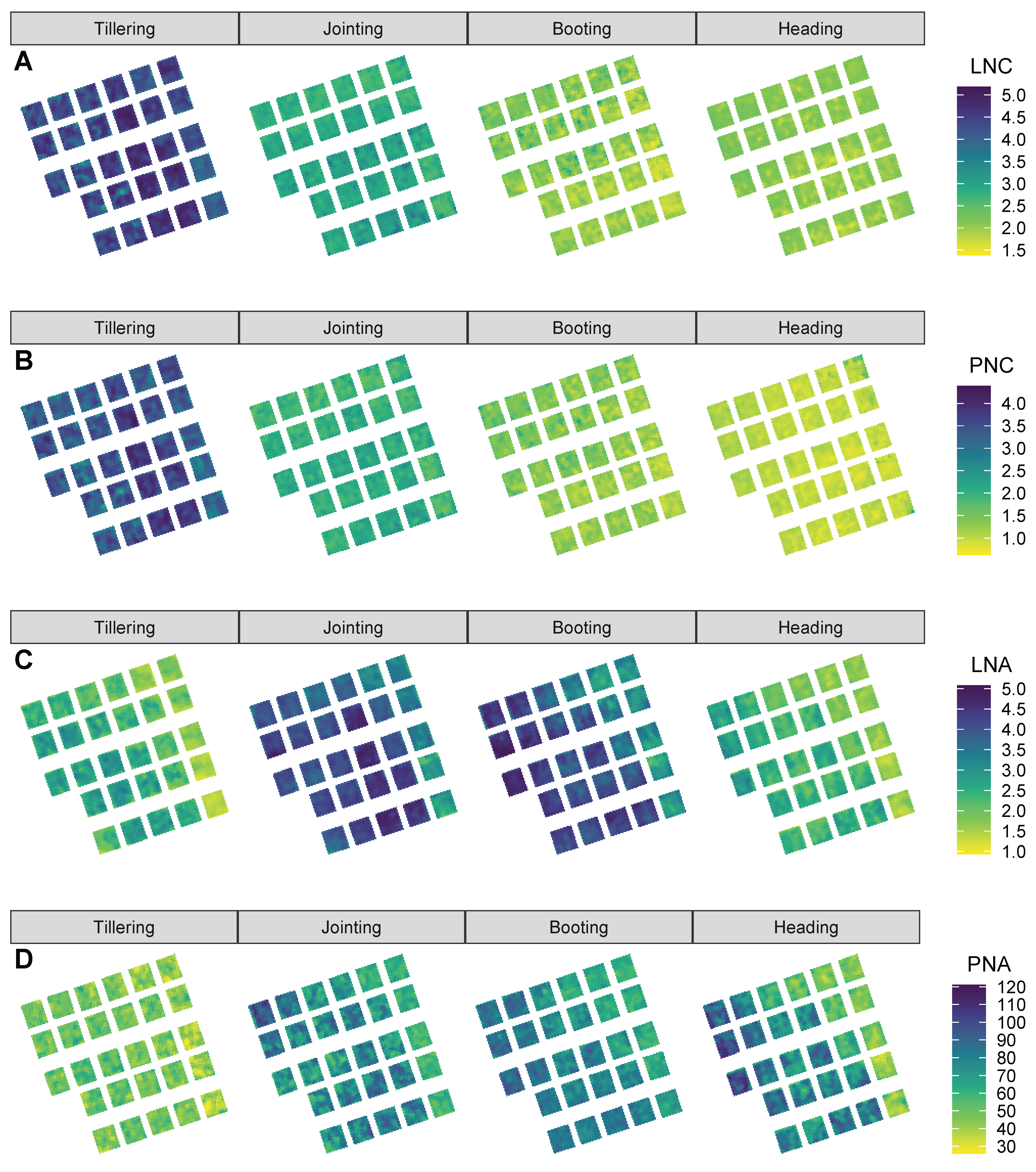
3.4. Evaluation on Hyperspectral Imageries

Figure 8 shows the pixelwise inversion results of the four N traits (LNC, PNC, LNA and PNC), using the corresponding optimal ML full-growth-stage models listed in Table 4 (the ANN for LNC and PNC and the SVM for LNA and PNA). The N treatment level variation is relatively homogenous. The spatial pattern due to different nitrogen treatments is more obvious in the maps of LNA and PNA than those of LNC and PNC. The N trait variations caused by growth stages are in line with the observations (detailed in Table 2).

4. Discussion

With a focus on fresh leaves or plant canopies instead of dry leaves or dried and ground leaves, the remote sensing-based estimation of nitrogen traits is mainly based on the relationship between chlorophyll and nitrogen by means of the use of visible and near infrared (VNIR) spectra. The pairwise correlation analysis (Figure 3) shows that the relationships among the four nitrogen traits and those between the four nitrogen traits and the three biochemical traits (LCC, CCC and ABG) are obviously affected by the growth stage, except for the relationship between LNC and PNC. During the vegetative growth stage, N is abundant in the vegetative tissues, while in the reproductive growth stage, N reallocates from the leaves to the reproductive organs (ears, fruits or seeds). In the reallocation process, the assembly and disassembly of N are accompanied by canopy structure variation. Additionally, the ABG increases more slowly with growth stage development, and the “dilution effects” end at the heading growth stage when the plant N content dominates the canopy reflectance [64]. The reallocation of N and variation in the biomass increase the rate change of the relationships between nitrogen and chlorophyll or ABG across the growth stages.
The performance of the growth-stage-specific VI-based nitrogen trait estimation models is relatively constant within the same growth stage. A similar pattern was observed in a previous study [15]. Patel et al. [15] evaluated the performance of several VIs for irrigated perennial ryegrass PNC estimation and found that the selected VIs showed a similar correlation with PNC when applied to single growth stage data. When multiple growth stage data were pooled together, the accuracy of VI-based full-growth-stage models degraded obviously. Li et al. [16] and Patel et al. [15] found similar results. This is because, in addition to the nitrogen and chlorophyll content, canopy reflectance is affected by LAI, ABG, nonphotosynthetic components, soil background and other factors. With the growth stage development, the canopy structure and background situation vary. The VIs that use several bands cannot fully capture the intrinsic relationship between the canopy spectrum and the target variable across growth stages.
There is general interest in exploring the red-edge spectrum, which are bands where reflectance sharply increases from the lower reflectance red region to high reflectance near the infrared region, for biochemical parameter estimation [13,25,28,64,65]. The REP, which is the main inflection point of the red-edge spectrum, has been found to be useful for chlorophyll and nitrogen content estimation. In this work, the REPs calculated with different techniques, such as linear four-point interpolation, linear extrapolation and Gaussian fit, were evaluated. Despite taking advantage of the narrower continuing hyperspectral data, the REPs are not obviously superior to other VIs in either growth-stage-specific or full-growth-stage models. However, there are several VIs that use the red-edge band—such as CIre, mND705, NDPI, and D735—that perform better than other VIs. Several works have pointed out the importance of blue bands for dry-mass-based nitrogen content (LNC and PNC) estimation [16,19,24]; however, our sensor does not cover this region.
Compared to the VI-based models, the PLSR and ML models generally yield better performance for the full-growth-stage models. This may be because more bands are involved, and the full potential of the hyperspectral data is explored. For the growth-stage-specific models, the PLSR and ML models generally show similar performance to, or even worse performance than, the corresponding VI-based models. This may indicate that for growth-stage-specific models, the VI-based estimation is optimal and cannot be further improved.

5. Conclusions

This work evaluates the performance of univariate regression model vegetation indices (VIs), traditional multivariate calibration method partial least squares regression (PLSR) and modern machine learning (ML) methods, such as the artificial neural network (ANN), random forest (RF), and support vector machine (SVM), for paddy rice nitrogen trait—leaf nitrogen content (LNC), plant nitrogen content (PNC), leaf nitrogen accumulation (LNA) and plant nitrogen accumulation (PNA)—estimation, with a special focus on the effects of growth stages. All methods were evaluated both throughout the growing season and at each growth stage (tillering, jointing, booting and heading).
The results indicate that the correlations between the four nitrogen traits and the other three biochemical traits—leaf chlorophyll content (LCC), canopy chlorophyll content (CCC) and aboveground biomass (ABG)—are affected by the growth stage. Within a single growth stage, the performance of the selected VIs is relatively constant. For full-growth-stage models, the performance of the VI-based models is more diverse. For full-growth-stage models, the TCARI/OSAVI performed best for LNC, PNC and PNA estimation, while the TBVITian performed best for LNA estimation. There are no obvious patterns showing whether the PLSR, ANN, RF or SVM performs best in either the growth-stage-specific or full-growth-stage models.
For the growth-stage-specific models, a lower MRE and higher R2 can be acquired at the tillering and jointing growth stages. The PLSR and ML methods yield obviously better estimation accuracy for the full-growth-stage models than the VI-based models. For the growth-stage-specific models, the performance of VI-based models seems optimal and cannot be obviously improved. These results suggest that building linear regression models on VIs for paddy rice nitrogen traits estimation is still a reasonable choice when only a single growth stage is involved. However, when multiple growth stages are involved or the phenology information is missing, using PLSR or ML methods is a better option. Nevertheless, it must be noticed that only one paddy rice variety was tested in our study. Whether our conclusions still hold when other varieties/cultivations or multiple varieties/cultivations are involved needs further evaluation.

Author Contributions

Conceptualization, L.W. and D.L.; methodology, L.W.; software, L.W.; validation, L.W.; formal analysis, L.W.; investigation, L.W., D.L., Z.P., C.W., H.J. and Q.Z.; resources, L.W.; data curation, L.W.; writing—original draft preparation, L.W.; writing—review and editing, D.L., C.W. and S.C.; visualization, L.W.; supervision, S.C.; project administration, S.C. and L.W.; funding acquisition, S.C. and L.W. All authors have read and agreed to the published version of the manuscript.

Funding

This research was funded by GDAS Project of Science and Technology Development (2020GDASYL-20200103011), Guangdong Province Agricultural Science and Technology Innovation and Promotion Project (No. 2021KJ102, No. 2020KJ102, No. 2019KJ102); Guangzhou Basic Research Project (202002020076).

Institutional Review Board Statement

Not applicable.

Informed Consent Statement

Not applicable.

Data Availability Statement

Data sharing is not application to this article.

Conflicts of Interest

The authors declare no conflict of interest.

References

  1. Berger, K.; Verrelst, J.; Féret, J.B.; Wang, Z.; Wocher, M.; Strathmann, M.; Danner, M.; Mauser, W.; Hank, T. Crop nitrogen monitoring: Recent progress and principal developments in the context of imaging spectroscopy missions. Remote Sens. Environ. 2020, 242, 111758. [Google Scholar] [CrossRef]
  2. Kokaly, R.F.; Asner, G.P.; Ollinger, S.V.; Martin, M.E.; Wessman, C.A. Characterizing canopy biochemistry from imaging spectroscopy and its application to ecosystem studies. Remote Sens. Environ. 2009, 113, S78–S91. [Google Scholar] [CrossRef]
  3. Li, D.; Zhang, P.; Chen, T.; Qin, W. Recent Development and Challenges in Spectroscopy and Machine Vision Technologies for Crop Nitrogen Diagnosis: A Review. Remote Sens. 2020, 12, 2578. [Google Scholar] [CrossRef]
  4. Lemaire, G.; Jeuffroy, M.H.; Gastal, F. Diagnosis tool for plant and crop N status in vegetative stage. Eur. J. Agron. 2008, 28, 614–624. [Google Scholar] [CrossRef]
  5. Chlingaryan, A.; Sukkarieh, S.; Whelan, B. Machine learning approaches for crop yield prediction and nitrogen status estimation in precision agriculture: A review. Comput. Electron. Agric. 2018, 151, 61–69. [Google Scholar] [CrossRef]
  6. Onojeghuo, A.O.; Blackburn, G.A.; Huang, J.; Kindred, D.; Huang, W. Applications of satellite ‘hyper-sensing’ in Chinese agriculture: Challenges and opportunities. Int. J. Appl. Earth Obs. Geoinf. 2018, 64, 62–86. [Google Scholar] [CrossRef] [Green Version]
  7. Pancorbo, J.; Camino, C.; Alonso-Ayuso, M.; Raya-Sereno, M.; Gonzalez-Fernandez, I.; Gabriel, J.; Zarco-Tejada, P.; Quemada, M. Simultaneous assessment of nitrogen and water status in winter wheat using hyperspectral and thermal sensors. Eur. J. Agron. 2021, 127, 126287. [Google Scholar] [CrossRef]
  8. Huang, Z.; Turner, B.J.; Dury, S.J.; Wallis, I.R.; Foley, W.J. Estimating foliage nitrogen concentration from HYMAP data using continuum removal analysis. Remote Sens. Environ. 2004, 93, 18–29. [Google Scholar] [CrossRef]
  9. Yang, G.; Zhao, C.; Pu, R.; Feng, H.; Li, Z.; Li, H.; Sun, C. Leaf nitrogen spectral reflectance model of winter wheat ( Triticum aestivum ) based on PROSPECT: Simulation and inversion. J. Appl. Remote Sens. 2015, 9, 095976. [Google Scholar] [CrossRef]
  10. Berger, K.; Verrelst, J.; Féret, J.B.; Hank, T.; Wocher, M.; Mauser, W.; Camps-Valls, G. Retrieval of aboveground crop nitrogen content with a hybrid machine learning method. Int. J. Appl. Earth Obs. Geoinf. 2020, 92, 102174. [Google Scholar] [CrossRef]
  11. Jacquemoud, S.; Baret, F. PROSPECT: A model of leaf optical properties spectra. Remote Sens. Environ. 1990, 34, 75–91. [Google Scholar] [CrossRef]
  12. Baret, F.; Houles, V.; Guerif, M. Quantification of plant stress using remote sensing observations and crop models: The case of nitrogen management. J. Exp. Bot. 2006, 58, 869–880. [Google Scholar] [CrossRef] [Green Version]
  13. Tian, Y.; Yao, X.; Yang, J.; Cao, W.; Zhu, Y. Extracting Red Edge Position Parameters from Ground- and Space-Based Hyperspectral Data for Estimation of Canopy Leaf Nitrogen Concentration in Rice. Plant Prod. Sci. 2011, 14, 270–281. [Google Scholar] [CrossRef]
  14. Li, F.; Mistele, B.; Hu, Y.; Yue, X.; Yue, S.; Miao, Y.; Chen, X.; Cui, Z.; Meng, Q.; Schmidhalter, U. Remotely estimating aerial N status of phenologically differing winter wheat cultivars grown in contrasting climatic and geographic zones in China and Germany. Field Crop. Res. 2012, 138, 21–32. [Google Scholar] [CrossRef]
  15. Patel, M.K.; Ryu, D.; Western, A.W.; Suter, H.; Young, I.M. Which multispectral indices robustly measure canopy nitrogen across seasons: Lessons from an irrigated pasture crop. Comput. Electron. Agric. 2021, 182, 106000. [Google Scholar] [CrossRef]
  16. Li, F.; Miao, Y.; Hennig, S.D.; Gnyp, M.L.; Chen, X.; Jia, L.; Bareth, G. Evaluating hyperspectral vegetation indices for estimating nitrogen concentration of winter wheat at different growth stages. Precis. Agric. 2010, 11, 335–357. [Google Scholar] [CrossRef]
  17. Fitzgerald, G.; Rodriguez, D.; Leary, G.O. Measuring and predicting canopy nitrogen nutrition in wheat using a spectral index—The canopy chlorophyll content index ( CCCI ). Field Crops Res. 2010, 116, 318–324. [Google Scholar] [CrossRef]
  18. Lee, Y.J.; Yang, C.M.; Chang, K.W.; Shen, Y. A Simple Spectral Index Using Reflectance of 735 nm to Assess Nitrogen Status of Rice Canopy. Agron. J. 2008, 100, 205–212. [Google Scholar] [CrossRef]
  19. Stroppiana, D.; Boschetti, M.; Brivio, P.A.; Bocchi, S. Plant nitrogen concentration in paddy rice from field canopy hyperspectral radiometry. Field Crop. Res. 2009, 111, 119–129. [Google Scholar] [CrossRef]
  20. Tian, Y.C.; Yao, X.; Yang, J.; Cao, W.X.; Hannaway, D.B.; Zhu, Y. Assessing newly developed and published vegetation indices for estimating rice leaf nitrogen concentration with ground- and space-based hyperspectral reflectance. Field Crops Res. 2011, 120, 299–310. [Google Scholar] [CrossRef]
  21. Wang, L.; Chang, Q.; Li, F.; Yan, L.; Huang, Y.; Wang, Q.; Luo, L. Effects of Growth Stage Development on Paddy Rice Leaf Area Index Prediction Models. Remote Sens. 2019, 11, 361. [Google Scholar] [CrossRef] [Green Version]
  22. Moharana, S.; Dutta, S. Spatial variability of chlorophyll and nitrogen content of rice from hyperspectral imagery. ISPRS J. Photogramm. Remote Sens. 2016, 122, 17–29. [Google Scholar] [CrossRef]
  23. Verrelst, J.; Malenovský, Z.; Van der Tol, C.; Camps-Valls, G.; Gastellu-Etchegorry, J.P.; Lewis, P.; North, P.; Moreno, J. Quantifying Vegetation Biophysical Variables from Imaging Spectroscopy Data: A Review on Retrieval Methods. Surv. Geophys. 2019, 40, 589–629. [Google Scholar] [CrossRef] [Green Version]
  24. Hansen, P.M.; Schjoerring, J.K. Reflectance measurement of canopy biomass and nitrogen status in wheat crops using normalized difference vegetation indices and partial least squares regression. Remote Sens. Environ. 2003, 86, 542–553. [Google Scholar] [CrossRef]
  25. Li, F.; Mistele, B.; Hu, Y.; Chen, X.; Schmidhalter, U. Reflectance estimation of canopy nitrogen content in winter wheat using optimised hyperspectral spectral indices and partial least squares regression. Eur. J. Agron. 2014, 52, 198–209. [Google Scholar] [CrossRef]
  26. Onoyama, H.; Ryu, C.; Suguri, M.; Iida, M. Nitrogen prediction model of rice plant at panicle initiation stage using ground-based hyperspectral imaging: Growing degree-days integrated model. Precis. Agric. 2015, 16, 558–570. [Google Scholar] [CrossRef]
  27. Yao, X.; Huang, Y.; Shang, G.; Zhou, C.; Cheng, T.; Tian, Y.; Cao, W.; Zhu, Y. Evaluation of six algorithms to monitor wheat leaf nitrogen concentration. Remote Sens. 2015, 7, 14939–14966. [Google Scholar] [CrossRef] [Green Version]
  28. Huang, S.; Miao, Y.; Yuan, F.; Gnyp, M.; Yao, Y.; Cao, Q.; Wang, H.; Lenz-Wiedemann, V.; Bareth, G. Potential of RapidEye and WorldView-2 Satellite Data for Improving Rice Nitrogen Status Monitoring at Different Growth Stages. Remote Sens. 2017, 9, 227. [Google Scholar] [CrossRef] [Green Version]
  29. Wang, B.; Chen, J.; Ju, W.; Qiu, F.; Zhang, Q.; Fang, M.; Chen, F. Limited Effects of Water Absorption on Reducing the Accuracy of Leaf Nitrogen Estimation. Remote Sens. 2017, 9, 291. [Google Scholar] [CrossRef] [Green Version]
  30. Li, F.; Wang, L.; Liu, J.; Wang, Y.; Chang, Q. Evaluation of Leaf N Concentration in Winter Wheat Based on Discrete Wavelet Transform Analysis. Remote Sens. 2019, 11, 1331. [Google Scholar] [CrossRef] [Green Version]
  31. Marang, I.J.; Filippi, P.; Weaver, T.B.; Evans, B.J.; Whelan, B.M.; Bishop, T.F.A.; Murad, M.O.F.; Al-Shammari, D.; Roth, G. Machine Learning Optimised Hyperspectral Remote Sensing Retrieves Cotton Nitrogen Status. Remote Sens. 2021, 13, 1428. [Google Scholar] [CrossRef]
  32. Nigon, T.; Yang, C.; Dias Paiao, G.; Mulla, D.; Knight, J.; Fernández, F. Prediction of Early Season Nitrogen Uptake in Maize Using High-Resolution Aerial Hyperspectral Imagery. Remote Sens. 2020, 12, 1234. [Google Scholar] [CrossRef] [Green Version]
  33. Zheng, H.; Li, W.; Jiang, J.; Liu, Y.; Cheng, T.; Tian, Y.; Zhu, Y.; Cao, W.; Zhang, Y.; Yao, X. A Comparative Assessment of Different Modeling Algorithms for Estimating Leaf Nitrogen Content in Winter Wheat Using Multispectral Images from an Unmanned Aerial Vehicle. Remote Sens. 2018, 10, 2026. [Google Scholar] [CrossRef] [Green Version]
  34. Yi, Q.; Huang, J.; Wang, F.; Wang, X. Evaluating the performance of PC-ANN for the estimation of rice nitrogen concentration from canopy hyperspectral reflectance. Int. J. Remote Sens. 2010, 31, 931–940. [Google Scholar] [CrossRef]
  35. Wang, F.; Huang, J.; Wang, Y.; Liu, Z.; Zhang, F. Estimating nitrogen concentration in rape from hyperspectral data at canopy level using support vector machines. Precis. Agric. 2013, 14, 172–183. [Google Scholar] [CrossRef]
  36. Guo, J.; Zhang, J.; Xiong, S.; Zhang, Z.; Wei, Q.; Zhang, W.; Feng, W.; Ma, X. Hyperspectral assessment of leaf nitrogen accumulation for winter wheat using different regression modeling. Precis. Agric. 2021, 1–25. [Google Scholar] [CrossRef]
  37. Wang, L.; Zhou, X.; Zhu, X.; Guo, W. Estimation of leaf nitrogen concentration in wheat using the MK-SVR algorithm and satellite remote sensing data. Comput. Electron. Agric. 2017, 140, 327–337. [Google Scholar] [CrossRef]
  38. Sun, J.; Yang, J.; Shi, S.; Chen, B.; Du, L.; Gong, W.; Song, S. Estimating Rice Leaf Nitrogen Concentration: Influence of Regression Algorithms Based on Passive and Active Leaf Reflectance. Remote Sens. 2017, 9, 951. [Google Scholar] [CrossRef] [Green Version]
  39. Dunn, B.; Dehaan, R.; Schmidtke, L.; Dunn, T.; Meder, R. Using Field-Derived Hyperspectral Reflectance Measurement to Identify the Essential Wavelengths for Predicting Nitrogen Uptake of Rice at Panicle Initiation. J. Infrared Spectrosc. 2016, 24, 473–483. [Google Scholar] [CrossRef]
  40. Zhao, H.; Song, X.; Yang, G.; Li, Z.; Zhang, D.; Feng, H. Monitoring of Nitrogen and Grain Protein Content in Winter Wheat Based on Sentinel-2A Data. Remote Sens. 2019, 11, 1724. [Google Scholar] [CrossRef] [Green Version]
  41. Moldenhauer, K.; Slaton, N. Rice growth and development. Rice Prod. Handb. 2001, 192, 7–14. [Google Scholar]
  42. Cerovic, Z.G.; Masdoumier, G.; Ghozlen, N.B.; Latouche, G. A new optical leaf-clip meter for simultaneous non-destructive assessment of leaf chlorophyll and epidermal flavonoids. Physiol. Plant. 2012, 146, 251–260. [Google Scholar] [CrossRef] [PubMed]
  43. Awais, M.; Li, W.; Cheema, M.J.M.; Hussain, S.; AlGarni, T.S.; Liu, C.; Ali, A. Remotely sensed identification of canopy characteristics using UAV-based imagery under unstable environmental conditions. Environ. Technol. Innov. 2021, 22, 101465. [Google Scholar] [CrossRef]
  44. Li, M.; Shamshiri, R.R.; Schirrmann, M.; Weltzien, C. Impact of Camera Viewing Angle for Estimating Leaf Parameters of Wheat Plants from 3D Point Clouds. Agriculture 2021, 11, 563. [Google Scholar] [CrossRef]
  45. Tian, M.; Ban, S.; Chang, Q.; Ma, W.; Yin, Z.; Wang, L. Estimation of SPAD value of cotton leaf using hyperspectral images from UAV-based imaging spectroradiometer. Trans. Chin. Soc. Agric. Eng. 2016, 47, 285–293. [Google Scholar]
  46. R Core Team. R: A Language and Environment for Statistical Computing; R Foundation for Statistical Computing: Vienna, Austria, 2021. [Google Scholar]
  47. Kuhn, M. plsmod: Model Wrappers for Projection Methods. R Package Version 0.1.1. 2020. Available online: https://github.com/tidymodels/plsmod (accessed on 1 January 2021).
  48. Venables, W.N.; Ripley, B.D. Modern Applied Statistics with S, 4th ed.; Springer: New York, NY, USA, 2002; ISBN 0-387-95457-0. [Google Scholar]
  49. Liaw, A.; Wiener, M. Classification and Regression by randomForest. R News 2002, 2, 18–22. [Google Scholar]
  50. Karatzoglou, A.; Smola, A.; Hornik, K.; Zeileis, A. kernlab—An S4 Package for Kernel Methods in R. J. Stat. Softw. 2004, 11, 1–20. [Google Scholar] [CrossRef] [Green Version]
  51. Clarke, T.R.; Moran, M.S.; Barnes, E.M.; Pinter, P.J.; Qi, J. Planar domain indices: A method for measuring a quality of a single component in two-component pixels. Int. Geosci. Remote Sens. Symp. 2001, 3, 1279–1281. [Google Scholar] [CrossRef]
  52. Tucker, C.J. Red and photographic infrared linear combinations for monitoring vegetation. Remote Sens. Environ. 1979, 8, 127–150. [Google Scholar] [CrossRef] [Green Version]
  53. Huete, A. A soil-adjusted vegetation index (SAVI). Remote Sens. Environ. 1988, 25, 295–309. [Google Scholar] [CrossRef]
  54. Rondeaux, G.; Steven, M.; Baret, F. Optimization of soil-adjusted vegetation indices. Remote Sens. Environ. 1996, 55, 95–107. [Google Scholar] [CrossRef]
  55. Qi, J.; Chehbouni, A.; Huete, A.R.; Kerr, Y.H.; Sorooshian, S. A modified soil adjusted vegetation index. Remote Sens. Environ. 1994, 48, 119–126. [Google Scholar] [CrossRef]
  56. Gitelson, A.a.; Gritz, Y.; Merzlyak, M.N. Relationships between leaf chlorophyll content and spectral reflectance and algorithms for non-destructive chlorophyll assessment in higher plant leaves. J. Plant Physiol. 2003, 160, 271–282. [Google Scholar] [CrossRef] [PubMed]
  57. Sims, D.A.; Gamon, J.A. Relationships between leaf pigment content and spectral reflectance across a wide range of species, leaf structures and developmental stages. Remote Sens. Environ. 2002, 81, 337–354. [Google Scholar] [CrossRef]
  58. Haboudane, D.; Miller, J.R.; Tremblay, N.; Zarco-Tejada, P.J.; Dextraze, L. Integrated narrow-band vegetation indices for prediction of crop chlorophyll content for application to precision agriculture. Remote Sens. Environ. 2002, 81, 416–426. [Google Scholar] [CrossRef]
  59. Wu, C.; Niu, Z.; Tang, Q.; Huang, W. Estimating chlorophyll content from hyperspectral vegetation indices: Modeling and validation. Agric. For. Meteorol. 2008, 148, 1230–1241. [Google Scholar] [CrossRef]
  60. Dash, J.; Curran, P.J. The MERIS terrestrial chlorophyll index. Int. J. Remote Sens. 2004, 25, 5403–5413. [Google Scholar] [CrossRef]
  61. Guyot, G.; Baret, F. Utilisation de la haute resolution spectrale pour suivre l’etat des couverts vegetaux. Spectr. Signat. Objects Remote Sens. 1988, 287, 279–286. [Google Scholar]
  62. Cho, M.A.; Skidmore, A.K. A new technique for extracting the red edge position from hyperspectral data: The linear extrapolation method. Remote Sens. Environ. 2006, 101, 181–193. [Google Scholar] [CrossRef]
  63. Miller, J.R.; Hare, E.W.; Wu, J. Quantitative characterization of the vegetation red edge reflectance 1. An inverted-Gaussian reflectance model. Int. J. Remote Sens. 1990, 11, 1755–1773. [Google Scholar] [CrossRef]
  64. Yu, K.; Li, F.; Gnyp, M.L.; Miao, Y.; Bareth, G.; Chen, X. Remotely detecting canopy nitrogen concentration and uptake of paddy rice in the Northeast China Plain. ISPRS J. Photogramm. Remote Sens. 2013, 78, 102–115. [Google Scholar] [CrossRef]
  65. Schlemmera, M.; Gitelson, A.; Schepersa, J.; Fergusona, R.; Peng, Y.; Shanahana, J.; Rundquist, D. Remote estimation of nitrogen and chlorophyll contents in maize at leaf and canopy levels. Int. J. Appl. Earth Obs. Geoinf. 2013, 25, 47–54. [Google Scholar] [CrossRef] [Green Version]
Figure 1. Demonstration of sample areas, nitrogen treatment leaves and hyperspectral camera setup. J0–J6 received 0, 30, 60, 90, 120, 150 and 180 (kg ha−1) nitrogen, respectively, at 7 DAT; F0–F6 each received 90 (kg ha−1) nitrogen at 7 DAT; F0–F6 received 0, 15, 30, 45, 60, 75 and 90 (kg ha−1) nitrogen, respectively, at 33 DAT. Each plot was equally split into two sampling areas. The red rectangles are the sampling area boundaries.
Remotesensing 13 02956 g001
Figure 2. General workflow of this study.
Remotesensing 13 02956 g002
Figure 3. Pairwise scatter plots and correlations of the observed LNC, PNC, LNA, PNA, LCC, CCC and ABG. The diagonal is the growth-stage-specific density plots of the corresponding traits. The left bottom is pairwise scatter plots. The upper right panel shows the pairwise full data set and growth-stage-specific correlation coefficients. *** stands for significance at the 0.001 level, ** stands for significance at the 0.01 level, and * stands for significance at the 0.05 level.
Remotesensing 13 02956 g003
Figure 4. Growth-stage-specific and full-growth-stage cross-validated MRE and R2 values of selected VIs for LNC, PNC, LNA and PNA prediction.
Remotesensing 13 02956 g004
Figure 5. Scatter plots between observed and predicted nitrogen traits in the validation data set of the models listed in Table 3. The gray line is the 1:1 line.
Remotesensing 13 02956 g005
Figure 6. Growth-stage-specific and full-growth-stage cross-validated MRE and R2 values of the PLSR, ANN, RF and SVM for LNC, PNC, LNA and PNA prediction.
Remotesensing 13 02956 g006
Figure 7. Scatter plots between observed and predicted nitrogen traits in the validation data set of the models listed in Table 4.
Remotesensing 13 02956 g007
Figure 8. Spatial mapping results for LNC (%, A), PNC (%, B), LNA (g m−1, C) and PNA (kg ha−1, D), using the corresponding optimal full-growth-stage ML models (the ANN for LNC and PNC, and the SVM for LNA and PNA, as listed in Table 4).
Remotesensing 13 02956 g008
Table 1. VIs evaluated in this study.
IndexDefinitionCite
NDVI ρ 800 ρ 670 ρ 800 + ρ 670 [52]
SAVI ( 1 + 0.5 ) ρ 800 ρ 670 ρ 800 + ρ 670 + 0.5 [53]
OSAVI ( 1 + 0.16 ) ρ 800 ρ 670 ρ 800 + ρ 670 + 0.16 [54]
MSAVI 2 ρ 800 + 1 ( 2 ρ 800 + 1 ) 2 8 ( ρ 800 ρ 670 ) 2 [55]
CIgreen ρ 800 ρ 560 1 [56]
CIre ρ 800 ρ 720 1 [56]
NDRE ρ 780 ρ 720 ρ 790 + ρ 720 [17]
D735 d R / d λ | 735 [18]
NDVI(483,503) ρ 503 ρ 483 ρ 503 + ρ 483 [19]
TBVItian ρ 705 ρ 717 + ρ 491 [20]
mND705 ρ 750 ρ 705 ρ 750 + ρ 705 + 2 × ρ 445 [57]
mSR705 ρ 750 ρ 445 ρ 705 ρ 445 [57]
TCARI 3 [ ( ρ 700 ρ 670 ) 0.2 ( ρ 700 ρ 550 ) ( ρ 700 / ρ 670 ) ] [58]
TCARI/OSAVI T C A R I O S A V I [58]
TCARI2 3 [ ( ρ 750 ρ 705 ) 0.2 ( ρ 750 ρ 550 ) ( ρ 750 / ρ 705 ) ] [59]
OSAVI2 ( 1 + 0.16 ) ρ 750 ρ 705 ρ 750 + ρ 705 + 0.16 [59]
TCARI2/OSAVI2 T C A R I 2 O S A V I 2 [59]
MTCI ( ρ 754 ρ 709 ) / ( ρ 709 ρ 681 ) [60]
REPLiREP through linear four-point interpolation[61]
REPLEREP through linear extrapolation[62]
mREIPREP through Gaussian fit[63]
CCCI N D R E m i n _ N D R E m a x _ N D R E m i n _ N D R E [17]
NDPI C I r e m i n _ C I r e m a x _ C I r e m i n _ C I r e [14]
ρ λ stands for the reflectance at band λ nm. If  λ does not match the S185 wavelengths, the mean reflectance of two adjacent bands is used. Considering that the λ = 445 nm band does not fall in the S185 band ranges, the closest band, λ = 450 nm, is used.
Table 2. Statistics of the observed LNC, %; PNC, %; LNA, g m−2; PNA, kg ha−1; LCC, μg cm−2; CCC, μg cm−2 and ABG, t ha−1. CV stands for the coefficient of variation.
Growth StageMinMaxMeanCV
LNCFull Data set1.415.162.6138.63
Tillering4.005.164.657.69
Jointing2.433.302.848.93
Booting1.412.331.8312.95
Heading1.772.322.076.52
PNCFull Data set0.834.151.7156.29
Tillering3.094.153.688.91
Jointing1.702.372.009.87
Booting0.881.491.1911.54
Heading0.831.201.019.90
LNAFull Data set1.126.413.4833.04
Tillering1.262.932.0524.21
Jointing2.896.414.2922.48
Booting2.415.783.9221.61
Heading1.124.232.6427.31
PNAFull Data set18.21156.3677.3439.58
Tillering18.2139.0028.0121.83
Jointing46.7595.5465.9619.91
Booting52.50115.9479.9817.79
Heading55.61141.8395.7220.64
LCCFull Data set22.3839.8830.6312.44
Tillering33.7839.8837.364.55
Jointing28.6735.4631.575.09
Booting25.2034.9228.557.38
Heading27.6934.3730.265.08
CCCFull Data set29.36293.72118.4551.89
Tillering32.7181.6356.2023.99
Jointing65.51201.15122.8127.85
Booting102.74293.72186.8523.35
Heading29.36127.6986.0326.14
ABGFull Data set0.5412.376.1054.24
Tillering0.540.980.7514.86
Jointing2.564.193.2813.54
Booting5.558.566.699.85
Heading6.6911.999.3613.43
Table 3. The goodness-of-fit of the best-performing VIs of the full-growth-stage and growth-stage-specific models for LNC, PNC, LNA and PNA selected according to MREcv.
CalibrationValidation
Data SetVegetation IndexMREcvRMSEcvR cv 2 MREvalRMSEvalR val 2
LNCFull Data setTCARI/OSAVI25.850.740.6224.950.680.61
TilleringCIgreen3.340.171.002.030.110.88
JointingREPLi3.800.121.004.060.130.87
BootingCIre10.000.200.5010.480.210.08
HeadingTCARI/OSAVI3.870.090.944.310.140.07
PNCFull Data setTCARI/OSAVI30.850.620.6925.180.530.73
TilleringCIgreen3.450.141.002.250.100.90
JointingmND7053.200.081.002.500.060.95
BootingNDPI6.060.090.655.090.080.50
HeadingmND7054.380.051.006.860.080.39
LNAFull Data setTBVITian16.910.610.7217.820.740.69
TilleringD7358.130.181.007.050.200.82
JointingOSAVI211.760.560.999.780.470.81
BootingNDPI14.100.630.6114.490.630.21
HeadingNDVI16.240.520.9915.010.450.28
PNAFull Data setTCARI/OSAVI12.4310.690.8416.7512.130.80
TilleringD7357.522.261.006.782.270.85
JointingNDRE10.387.821.009.986.700.79
BootingTCARI2/OSAVI28.197.750.749.5310.750.36
HeadingREPLE10.3011.441.0013.3513.940.51
Table 4. The goodness-of-fit values of the best-performing models of the full-growth-stage and each growth-stage-specific models for LNC, PNC, LNA and PNA selected by MREcv.
Calibration (Cross-Validated)Validation
Data SetMethodMREcvRMSEcv R cv 2 MREvalRMSEval R val 2
LNCFull Data setANN7.820.210.956.620.190.97
TilleringRF3.100.160.983.380.190.86
JointingSVM3.860.121.006.800.200.44
BootingPLSR11.420.230.158.760.190.50
HeadingSVM3.660.090.9410.540.250.01
PNCFull Data setANN6.410.120.985.150.110.99
TilleringPLSR3.020.120.982.560.120.90
JointingSVM3.030.071.004.650.110.80
BootingPLSR7.300.100.443.840.060.82
HeadingPLSR5.160.060.956.590.070.83
LNAFull Data setSVM14.850.600.7211.040.490.81
TilleringANN7.100.150.989.180.200.91
JointingPLSR11.090.530.9810.880.450.84
BootingANN14.590.670.5415.730.830.22
HeadingPLSR14.650.480.9928.260.550.88
PNAFull Data setSVM11.329.160.8411.1111.400.87
TilleringPLSR6.021.791.009.312.800.95
JointingRF9.796.880.999.327.540.69
BootingPLSR8.598.850.616.107.500.77
HeadingPLSR10.7111.660.9010.839.490.95
Publisher’s Note: MDPI stays neutral with regard to jurisdictional claims in published maps and institutional affiliations.

