
UAV Thermal Images for Water Presence Detection in a Mediterranean Headwater Catchment


1
Department of Environmental Engineering, University of Calabria, 87036 Rende, Italy
2
Department of Civil, Architectural and Environmental Engineering, University of Padua, 35131 Padua, Italy
*
Author to whom correspondence should be addressed.
Remote Sens. 2022, 14(1), 108; https://0-doi-org.brum.beds.ac.uk/10.3390/rs14010108
Submission received: 4 November 2021
/
Revised: 19 December 2021
/
Accepted: 22 December 2021
/
Published: 27 December 2021
(This article belongs to the Special Issue Advances in Remote Sensing for Environmental Monitoring)
Abstract
:As Mediterranean streams are highly dynamic, reconstructing space–time water presence in such systems is particularly important for understanding the expansion and contraction phases of the flowing network and the related hydro–ecological processes. Unmanned aerial vehicles (UAVs) can support such monitoring when wide or inaccessible areas are investigated. In this study, an innovative method for water presence detection in the river network based on UAV thermal infrared remote sensing (TIR) images supported by RGB images is evaluated using data gathered in a representative catchment located in Southern Italy. Fourteen flights were performed at different times of the day in three periods, namely, October 2019, February 2020, and July 2020, at two different heights leading to ground sample distances (GSD) of 2 cm and 5 cm. A simple methodology that relies on the analysis of raw data without any calibration is proposed. The method is based on the identification of the thermal signature of water and other land surface elements targeted by the TIR sensor using specific control matrices in the image. Regardless of the GSD, the proposed methodology allows active stream identification under weather conditions that favor sufficient drying and heating of the surrounding bare soil and vegetation. In the surveys performed, ideal conditions for unambiguous water detection in the river network were found with air–water thermal differences higher than 5 °C and accumulated reference evapotranspiration before the survey time of at least 2.4 mm. Such conditions were not found during cold season surveys, which provided many false water pixel detections, even though allowing the extraction of useful information. The results achieved led to the definition of tailored strategies for flight scheduling with different levels of complexity, the simplest of them based on choosing early afternoon as the survey time. Overall, the method proved to be effective, at the same time allowing simplified monitoring with only TIR and RGB images, avoiding any photogrammetric processes, and minimizing postprocessing efforts.
1. Introduction
The use of UAVs (Unmanned Aerial Vehicles) in the study and monitoring of the environment is growing exponentially, thanks also to the availability of equipment with increasingly versatile sensors of reduced size and weight. The possibility of significantly increasing the temporal and spatial resolution of the datasets, as compared to the satellite remote sensing platforms and manned aircraft [1], gives the UAVs an intermediate position between these platforms and land surveys. Moreover, this technique is relatively cheap to use and not particularly time consuming. The efficiency of drones for environmental surveys is widely demonstrated in the literature (e.g., [2,3,4,5]). Manfreda et al. [1], while discussing the most recent advances, pointed out the need to identify the limitations of these technologies, which often lack standard protocols unequivocally identifying all the procedural steps, starting from data acquisition up to the final products (e.g., maps, 3D models, and ortophotos, etc.).
The first scientific applications with UAVs mainly concerned photogrammetry with innovative Structure from Motion (SfM) techniques [6,7]. Afterwards, new sensors (thermal cameras, multispectral and hyperspectral cameras, and LiDAR) were adapted to UAVs and used for different purposes (environmental monitoring, precision farming, and forest fires, etc.) [8]. Specifically, several studies demonstrated the potential of this technology for monitoring and understanding river network dynamics (e.g., [8,9,10,11,12,13,14,15,16,17,18,19]). Among them, Tamminga et al. [10] and Woodget et al. [14] identified the advantages of UAV systems to characterize the morphologies of hydraulic channels using red–green–blue (RGB) photogrammetry with the SfM technique. Using a UAV system capable of capturing RGB, near–infrared (NIR), and thermal infrared (TIR) images, Jensen et al. [9] performed in–stream temperature measurements with high spatial and temporal resolutions. Specifically, they identified the water pixels using the NIR band, in which water has a very low reflectance compared to soil and vegetation, and they used the corresponding TIR images to measure water temperature. The advantages compared to ground surveys of using UAVs in river flow management are also described by Samboko et al. [18], who highlighted the potential of UAVs for monitoring dangerous and difficult to access reaches. However, the precise mapping of the geomorphic channel for the recognition of water pixels requires approaches based on the use of multiple sensors (e.g., RGB and TIR; Kuhn et al. [19]), further emphasizing the need for standardized methods in the analysis of UAV–gathered images.
Monitoring the presence of water in channels remotely with the use of drones is particularly useful in the study of the expansion and contraction dynamics of active river networks. The topic is experiencing a renewed interest of the scientific community owing to the influence of stream dynamics on hydrology, freshwater ecology, and biogeochemistry (e.g., [20,21,22]). In this context, the Mediterranean region is particularly challenging, owing to the enhanced variability of the active length in arid and semiarid regions [23,24]. Borg Galea et al. [16] showed the usefulness of drones for monitoring intermittent Mediterranean rivers using RGB images. However, the authors also highlighted the need to search for better solutions for space–time monitoring of the flow regimes in intermittent streams. Spence & Mengistu [12] comparatively evaluated the efficiency of high–resolution RGB images from UAVs to identify the active part of intermittent flowing networks. Rivas Casado et al. [25] also showed the importance of UAV image resolution for the correct identification of wet channels. This is true especially for narrow and highly dynamic headwater streams that experience several activation–deactivation cycles within the same hydrological year.
Water presence detection in surface water bodies is generally performed with multispectral images, acquired with RGB, NIR, and short wavelength infrared (SWIR) sensors, and relies on the calculation of normalized indices. Among these, the best known is the NDWI (Normalized Difference Water Index; McFeeters [26]), calculated as:
The identification of water pixels is then performed imposing a minimum threshold on the NDWI. The NDWI has been extensively used, especially in combination with satellite images (e.g., [27,28,29,30,31]), for mapping water bodies or quantifying surface water resources (e.g., [32,33,34,35]) and soil moisture (e.g., [36,37]). The NDWI underwent several modifications and revisions [27,38,39,40,41] aimed at overcoming its major shortcomings. One inherent limit of NIR images is that they cannot be used for spatially distributed water temperature monitoring but only for water presence detection.
To the best of our knowledge, the literature lacks detailed investigations about the possibility of detecting water presence in river channels using only TIR and RGB images, in the absence of NIR or SWIR sensors. The TIR–based remote sensing approach is based on the analysis of infrared radiation emitted by objects with a temperature greater than 0 Kelvin, measured with thermal imaging cameras. These instruments provide radiometric images to a single band, usually 16–bit (range of values 0–65.535), with pixel values (digital number DN) proportional to the TIR radiance. The temperature measured with the TIR technique is defined as radiometric temperature (Tr), to be distinguished from the real kinetic temperature (Tk) measured with conventional devices, such as thermometers and standard contact probes. TIR measurements are mainly conditioned by the emissivity (ε) and the reflectance (ρ) of the objects (the third component, i.e., the transmissivity τ, is usually negligible), which are, as per the well–known Kirchhoff’s law, inversely proportional:
Water has a low reflectance in the TIR band and consequently a very high emissivity [42], standing at values of about 0.98–0.99, therefore resulting in being essentially opaque.
Hancock et al. [43] recently summarized the state–of–the–art TIR technology for different types of applications in riverine landscapes. Dugdale et al. [44] demonstrated the efficiency of drone shooting images for characterizing the spatial patterns of river temperature. Casas–Mulet et al. [17] proposed a method that combines TIR and RGB images for the study of thermal contrasts in rivers, also hypothesizing that water can be detected using TIR images when sufficient contrast exists with the surrounding terrain. Kuhn et al. [19] used RGB and TIR images from UAVs for the identification and characterization of thermally differentiated patches to model how climatic predictions affect thermal habitat suitability and connectivity of a cold–adapted fish species; they also reiterated that the combined use of TIR and RGB images is still under development.
In this paper, the efficiency of UAV–based TIR remote sensing technology in recognizing water pixels, as an alternative to the use of multispectral image sets, is tested for the first time. TIR–based techniques are increasingly used in many research and applicative fields, owing to the increased reliability, stability, portability, and affordability of TIR imaging systems. The use of TIR images for both water pixel detection and spatially distributed water temperature measurements would greatly simplify postprocessing operations, with a reduced number of IR images to be georeferenced and managed. The main purpose of the paper is to evaluate the effectiveness of TIR technology for water pixel detection based on combined TIR and RGB images only. The procedure allows one to leave out all issues related to TIR image calibration and accuracy evaluation of the radiometric temperature measurements since the method exploits only the thermal contrast (temperature gradient) between water and the surrounding environment.
The main aim was pursued by performing several sample flights over a Mediterranean headwater channel using a UAV equipped with RGB and thermal sensors. The selected location, although representative of many Mediterranean headwaters, was particularly challenging since it is characterized by a narrow flowing section (minimum width of 1 m) and a dense vegetation cover. With the goal of exploring the broadest range of climate and vegetation conditions and testing different image resolutions, the flights were carried out during different seasons, times, and heights. The accuracy of the results was evaluated accounting for the observed water temperature, suitably measured with a thermometric probe, and several meteorological variables. Eventually, a method was proposed for the detection of the water pixels within the surveyed channel using only noncalibrated TIR images and a control point with the water presence verified by either a ground survey or with the support of RGB images.
2. Materials and Methods
2.1. Study Site
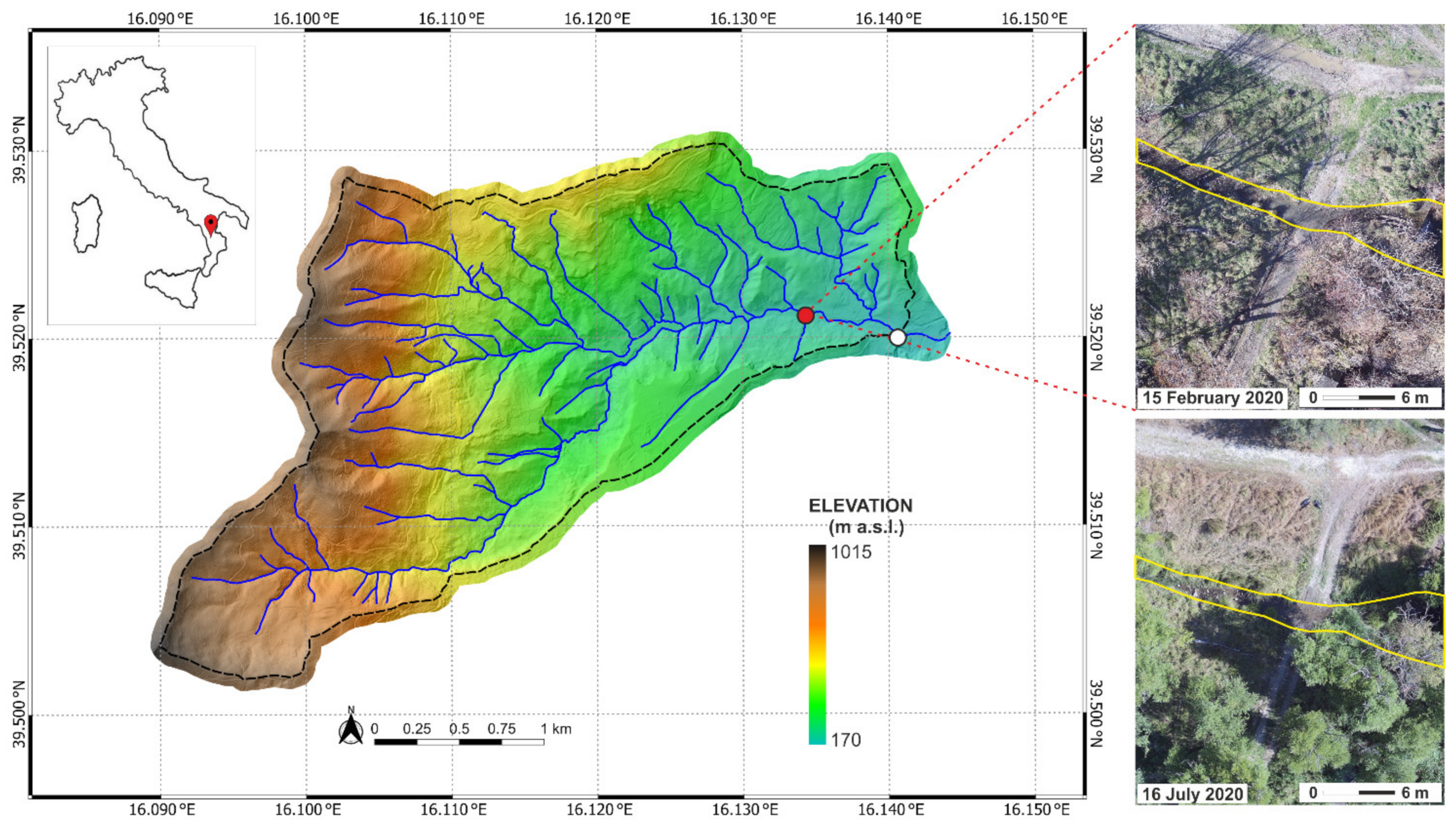
The surveys were carried out along a river reach some tens of meters long located approximately 550 m upstream of the outlet of the Upper Turbolo catchment [23] (Figure 1), Southern Italy. The catchment is 7 km2 wide, with altitudes ranging from 183 m a.s.l. at the outlet to 1005 m a.s.l. on top of the Coastal Range mountains. The complex lithology of the area implies a significant hydrogeological variability, with the presence of deep and free–surface aquifers feeding the main river network. As a consequence, despite a typically Mediterranean climate with long hot and dry summers [23], the measurements recorded at the Fitterizzi outlet (white dot in Figure 1) display a quasi–permanent hydrological regime.
The selected reach, located at 39.5214° N and 16.1346° E (200 m a.s.l.), is characterized by a width of the riverbed varying approximately from 1.0 m to 2.5 m and a gentle slope. The Thalweg elevation varies from 198.2 m a.s.l. to 197.8 m a.s.l. at the upstream and downstream sections of the 24 m long reach, respectively, leading to an approximate slope of 1.7% (a high–resolution 3D representation of the DTM of the whole area is represented in the Supplementary Materials Figure S1). As frequently observed in Mediterranean catchments, the riparian zone (i.e., the interface between the river reach and the surrounding territory) is mostly densely vegetated with hygrophilous vegetation (reeds, bushes, shrubs, and even trees–mainly alders, Alnus). However, some portions of the reach are visible both from above and from the ground, allowing for a direct visual inspection of the underlying hydrologic conditions. To generalize the analysis as much as possible, the reach was selected also for the presence of a ford, in correspondence of which the boundaries of the geomorphic channel are less sharp.
2.2. Instruments
For the experimental activities, a DJI drone model Matrice 200 V1 was used. It is a quadcopter equipped with high–performance engines and functions, capable of operating in various environmental and climatic conditions, thanks also to a compact and hermetically sealed design, it is resistant to weather and water. The weight of the aircraft (without payload) is approximately 4.1 kg, with a flight duration of up to approximately 30 min with a payload of 1.45 kg.
The images were taken with the DJI Zenmuse XT2, a camera equipped with a radiometric thermal sensor and an RGB sensor (Table 1). This camera takes synchronous thermal and RGB images. The two sensors have different resolution and optical–geometric characteristics. This difference, together with the slight physical distance between the two sensors, requires particular care for image overlay. For our analysis, the RGB images, having a FOV and resolution greater than thermal images, were preliminarily cropped to homogenize the areas represented by the two sensors and resampled according to the thermal sensor resolution to obtain the same GSD.
2.3. Field Data Collection
The surveys were carried out on three different dates, i.e., mid–season (22 October 2019), cold season (15 February 2020), and hot season (16 July 2020), to explore the broadest possible variety of weather conditions. Considering that the ground sample distance (GSD) depends on the optical–geometric characteristics of the sensor used and the distance between the sensor and the target (i.e., GSD = (pixel size × h)/f, with h = flight height and f = focal length of the chamber), two different heights, 22 m and 56 m, were used for image acquisition, leading to thermal GSDs of 2 cm and 5 cm, respectively, and RGB GSDs of 0.5 cm and 1.3 cm, respectively. Two flight altitudes were also used to evaluate potential conditioning on the radiance measurements due to atmospheric agents. Table 2 summarizes all the surveys acquisition data, while Supplementary Table S1 provides further information about weather conditions in the flight dates.
For each flight, the drone was first lifted to 22 m of altitude, and the image set was taken in nadiral, then, on the same vertical, to 56 m, and the other image set was taken. The flights were performed in manual driving mode, checking the altitudes directly on the drone controller, which allows a real–time control of the scene shot by both the RGB and TIR sensors, making it easier to frame the same area with both sensors. The altitude above ground was based on the operator’s location, which was the same for all surveys.
During the flights, the kinetic temperatures of the water and air were recorded. Water temperature was measured with a manual thermometric probe (YSI EXO2 sonde temperature sensor, having a resolution of 0.001 °C and an accuracy of ±0.2 °C), air temperature through the nearby Fitterizzi weather station (resolution of 0.1 °C, accuracy of ±0.2 °C) managed by the Regional Agency for the Protection of the Environment (ARPACal). This station also provided measurements of precipitation, air relative humidity and pressure, wind speed and direction, and solar radiation, from which reference evapotranspiration can also be calculated (Allen et al., 1998). Temperature data were used to define the thermal contrasts between water and air (Table 3) at the same time of acquisition of UAV images. Furthermore, we kept note of the presence of pools of stagnant water outside the geomorphic channel, but in the framed area, localizing them through cell phone GPS measurements.
2.4. Data Processing
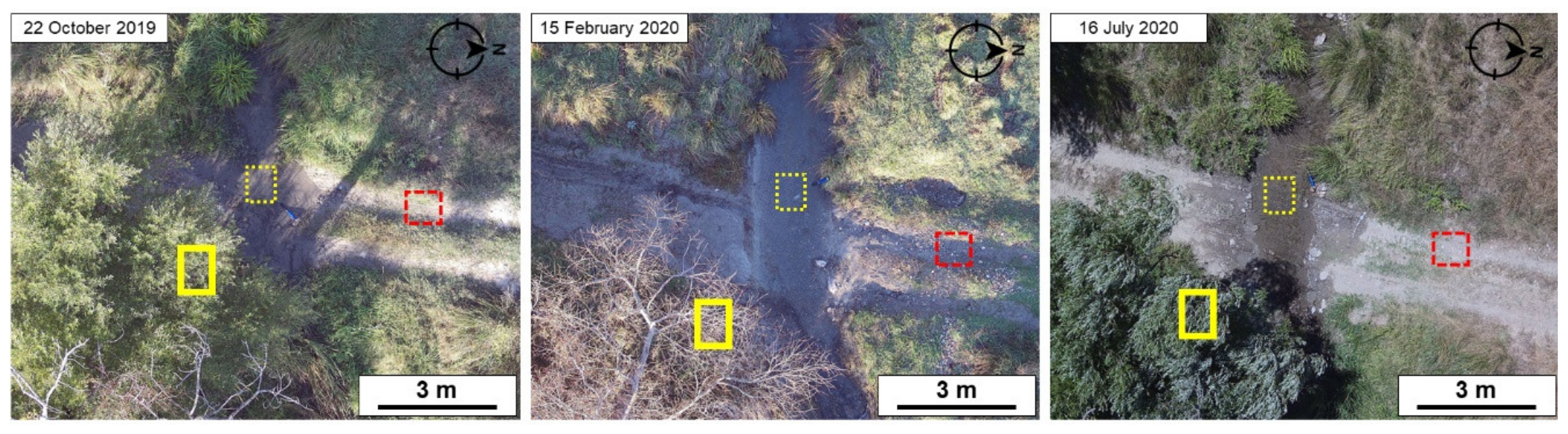
Each image set of thermal images, taken in 16–bit TIFF format, and RGB images was georeferenced on its own using the onboard GPS. Afterwards, the images were overlaid using the Quantum GIS open–source software. The RGB images were used to (a) support the direct surveys on the ground and allow the delimitation in the GIS environment of the morphological channel and (b) recognize sample areas with well–defined land cover. Specifically, for each RGB image, three as large as possible polygons were drawn enclosing as many homogenous land cover types (bare soil, vegetated soil, and water, respectively; Figure 2). Afterwards, the same polygons were overlaid to the TIR images, extracting as many ‘control matrices’, for which the ranges of DN values (from minimum to maximum) were calculated. Such ranges were assumed as representative of the thermal signatures of the three different land covers.
The drawing of the polygons followed criteria of simplicity and accuracy. To this aim, simple shapes (rectangles) were chosen, and the polygons were always located well inside their reference land cover types to prevent possible problems with imperfect georeferentiation with the UAV onboard GPS (which, in its turn, was preferred to more accurate georeferentiation with ground control points for the sake of simplicity). Further research could improve this basic yet flexible approach.
The DN ranges were compared considering different dates and flight heights and overlapped to the frequency distribution of the overall DN values in the images. Finally, the effectiveness of the DN ranges found in the water control matrices was evaluated in identifying water pixels in different seasons, day times and flight heights.
3. Results
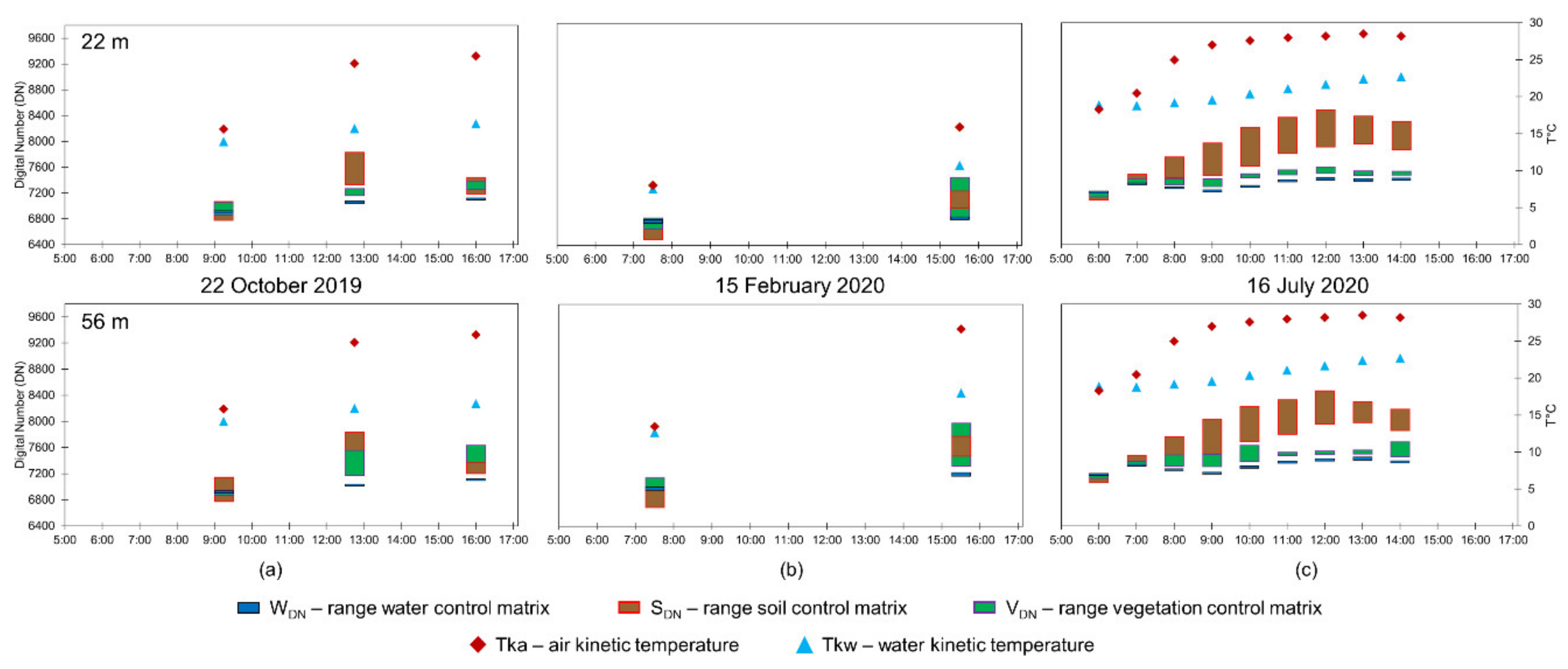
Figure 3 shows the time evolution of the DN range (min–max) of the control matrices of water (WDN), soil (SDN), and vegetation (VDN) and the kinetic temperatures of water and air measured for all 14 flights, subdivided for each of the three days of surveys and flight heights. During the first hours of daylight, water and air temperatures were always similar, and the WDN ranges overlaid to the VDN and SDN. Then, during the day, in October and July, surface heating due to radiation increased the air temperature more than water temperature, and the VDN and (mainly) SDN ranges were higher than the WDN, preventing any overlapping among the ranges of soil, water, and vegetation. In February, the air temperature gradient was still higher than water, but all the DN ranges overlapped, except for the WDN in the afternoon flight with 56 m height.
Table 4 summarizes the results of all the surveys carried out, distinguishing between the cases where the WDN ranges overlapped to the other DN ranges (O) or not (NO). The only situation with differences between flights at 22 m and 56 m occurs in the afternoon of the winter survey. While at 22 m the WDN maximum value skims the lowest value of the VDN range, at 56 m these two values are more clearly separated. This difference is an effect of the slightly different DN ranges captured at different GSDs. The Table also highlights the instances in which pixels falling in the WDN range were detected outside the geomorphic channel. These situations can be due either to the presence of pools and very humid areas, especially in the morning (true detection–TD), or to the similarity of the thermal signatures of water and vegetation/soil (false detection–FD).
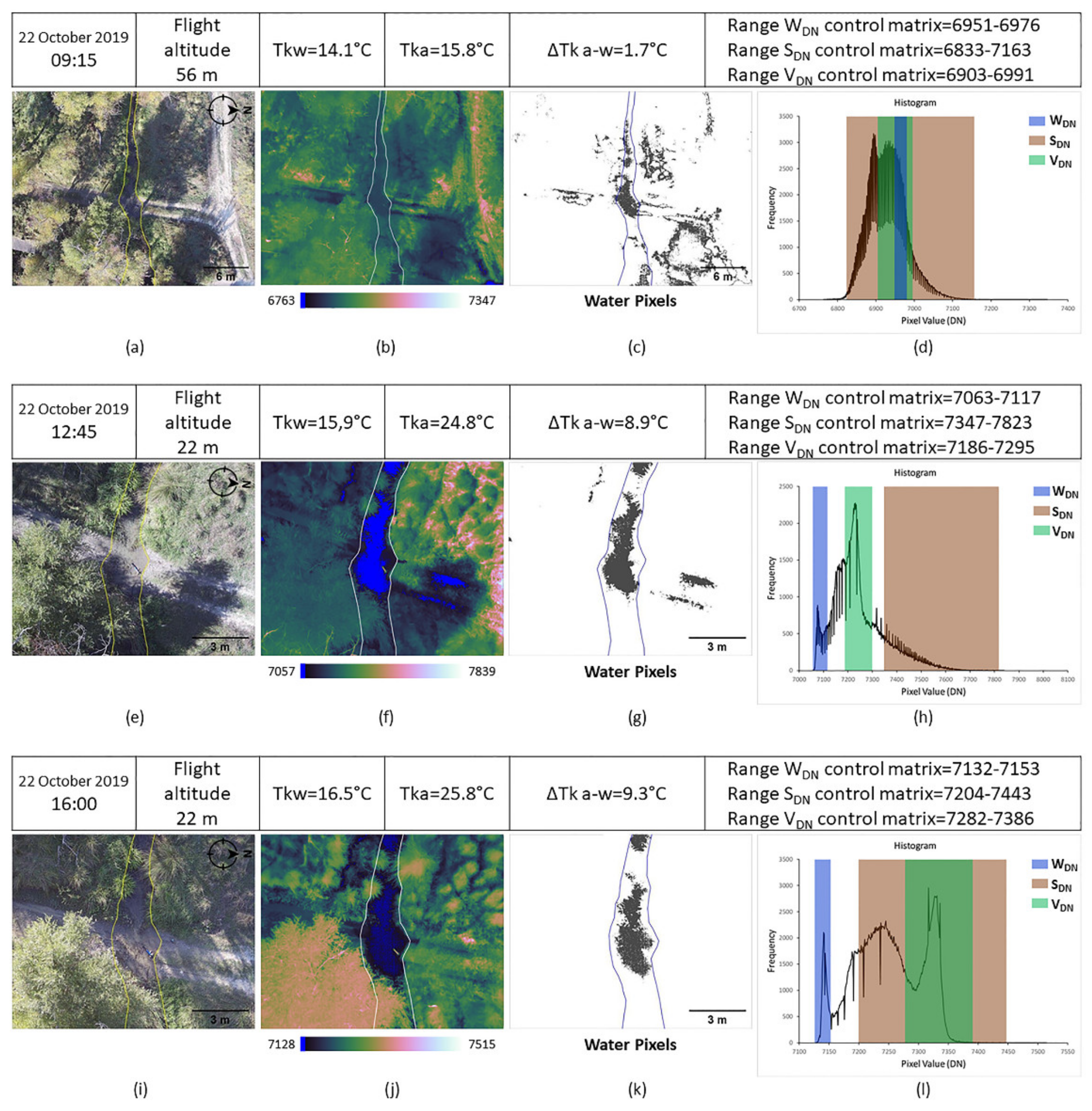
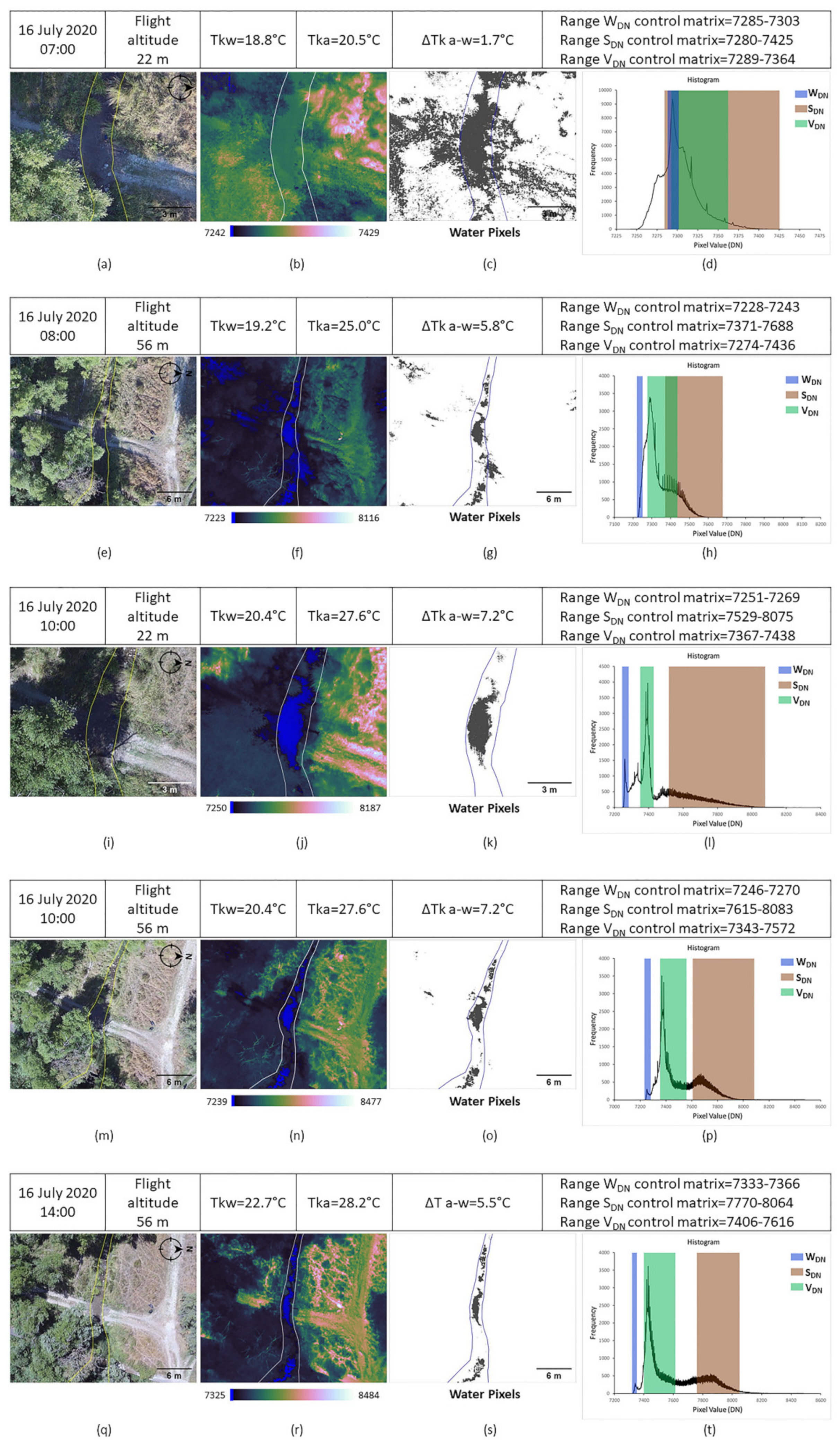
Figure 4, Figure 5 and Figure 6 show a set of representative examples of different situations observed during each of the three field surveys (all survey images are shown in the Supplementary Materials Figures S2–S13). Every Figure is composed of different panels, showing for the analyzed flights the following information: (i) the RGB image, with the delimitation of the geomorphic channel; (ii) the corresponding IR thermal image in false color, with the delimitation of the geomorphic channel; (iii) the pixels within the WDN range (water pixels, hereafter); (iv) the frequency distributions of the DN values of the thermal images, highlighting the WDN, SDN, and VDN ranges. Furthermore, information is provided about the date, time, and height of the flight; kinetic water and air temperatures and related difference (ΔTk a–w), and minimum and maximum values of the WDN, SDN, and VDN ranges.
In the survey carried out on 22 October 2019, the presence of water was unambiguously identified by extracting the pixels falling in the WDN range both in the second (performed at 12:45) and in the third (at 16:00) flights, while in the morning, flight several false detections occurred (Figure 4). This result was achieved regardless of the flight height.
In the morning flight, the low thermal contrast between the water and the surrounding environment (ΔTkaw = 1.7 °C, Table 3) determined an overlap of the water and soil/vegetation DN values, as highlighted by the DN frequency distributions shown in Figure 4d. Several shaded soil areas were incorrectly classified as water pixels, as shown by the comparison between Figure 4a,c. As the atmospheric temperature increased during the day, with consequent drying of soil and vegetation, the WDN range differentiated clearly from VDN and SDN ranges (Figure 4h,l), allowing more precise identification of water pixels, even outside the geomorphic channel. Figure 4e–h shows the results achieved at 12:45 with a flight height of 22 m, i.e., providing higher detail. The water pixels identified outside the channel (Figure 4f,g) are due to muddy (and therefore colder) bare soil areas, located in correspondence of the tires track of the ford crossing the reach. Such clusters can be easily discarded if the primary interest is detecting the active portion of the geomorphic network. The discontinuity of water pixels in the channel is due to the presence of vegetation that beclouds the thermal signature of the underlying water. The sections of the reach visible from the sensors can be assumed as river network active “nodes” (i.e., with the presence of water), as suggested by Durighetto et al. [22] and Senatore et al. [23]. If a stretch whose visibility is obstructed by vegetation is characterized upstream and downstream by active nodes, the whole stretch is likely active.
The image taking distances (i.e., the flight altitude) did not significantly affect the results, apart from the obvious impact on the resolution. Conversely, the level of signal noise recorded by the thermal sensor depending on the survey time should be considered: in the morning, operating at an air temperature of 15.8 °C (Table 3), the signal had a high noise level, with the frequencies of the DN values very close to each other and oscillating notably (Figure 4d). Such noise is significantly reduced in the surveys performed with warmer weather conditions (Figure 4h,l). This demonstrates the enhanced sensitivity of the microbolometric thermal sensors to the temperatures outside and inside the camera.
In the winter survey (15 February 2020), only two flights were performed (Figure 5). These flights were scheduled at times coinciding roughly with the minimum and maximum atmospheric temperature foreseen during daylight (07:30 and 15:30, respectively). In both cases, several water pixels outside the river network were detected by the developed algorithm. The incorrect classification can be attributed to different reasons. The conditions at the beginning of the day were generally moister than the previous survey, given a small rain event in the previous afternoon (almost 12 mm, Table S1). In the morning (07:30), the kinetic temperatures of the water and air were very similar (only 0.5 °C difference, Table 3). In such a context, the WDN range included the DN values in the upper percentiles of the overall frequency distribution of the observed SDN (Figure 5d), thereby overlapping the VDN range. At that time, the soil surface was not yet reached by sunbeams (Figure 5a), and it was generally colder than flowing water (Figure 5b), while vegetation started to heat. Accordingly, the detection of false water pixels mainly concerned vegetation pixels (Figure 5c). Nevertheless, some features concerning flowing water were correctly detected even outside the geomorphic channel. For example, the small rivulet entering the main course from its right bank (Figure 5c, probably an effect of the precipitation that occurred the previous day) represents real flowing water within the tire tracks of the ford. At 15:30, despite a temperature difference between air and water of 5.2 °C (Table 3), many soil and vegetation pixels were incorrectly classified as water pixels using the images taken during the flights performed at both 22 m and 56 m, despite in the last case the WDN range was not overlapped to the VDN and SDN. In both cases, the WDN range did not correspond to the lower (left hand side) values of the frequency distributions (Figure 5h,l). Lower DN values were associated with several shaded areas (especially vegetated) in the frame. As a result, water was correctly detected in the channel only around the control matrix, with many false detections in the surrounding regions. As regards the quality of the data collected by the sensor, due to the relatively low air temperatures, all the observed DN frequency distributions were very noisy.
The third survey was carried out on 16 July 2020, scheduled on an hourly basis from 06:00 to 14:00. The flights made at 06:00 and 07:00 broadly reproduced the same situation of the first surveys performed on 22 October 2019 and 15 February 2020, with low ΔTk a–w values (even negative at 06:00), overlapping of the WDN range with the VDN and SDN ranges, and several false water pixel detections (an example is given in Figure 6a–d). Then, the sudden increase in air temperature recorded from 07:00 to 08:00 (from 20.5 °C to 25.0 °C, Table 3 and Figure 3) quickly led to an air/water thermal contrast of 5.8 °C. The WDN range no longer overlapped to the VDN and SDN ranges and started to locate on the left end of the frequency distribution (e.g., Figure 6h), but some false detections outside the channel still occurred, both in the 22 m and 56 m flights. As Figure 6e–g show, false detections are due to the shadowed vegetated areas. The same example also shows some true detections along the tire tracks of the ford, with the presence of stagnant water, not yet dry.
The only slight difference between 22 m and 56 m flights was found at 10:00. At such time, while no water pixels outside the geomorphic channel were found in the higher–resolution scene (Figure 6i–l), the 56 m flight framing a wider area (Figure 6m–p) detected both true water pixels (i.e., the pools in the tire tracks of the ford) and few false water pixels (shadowed vegetation, the top left corner of Figure 6p). From 11:00 onwards, the drying of soil and vegetation facilitated a reliable distinction of the water pixels in the scene during all the performed flights (as shown in the example of Figure 6q–t). Neither true nor false water pixels outside the channel were detected, except for some small areas in correspondence of the ford where the geomorphic borders were slightly overcome (e.g., Supplementary Materials Figures S10–S12).
The quality of the thermal sensor signal on this day was quite variable, i.e., in the measurements taken from 06:00 to 09:00, with the atmospheric temperature varying from 18.3 to 25 °C, the frequency distributions were not very noisy (especially at 07:00, with an atmospheric temperature of 20.5 °C, Figure 6d). For the later surveys after 10:00, which were performed at atmospheric temperatures above 27 °C, the noise is more pronounced, as in the example of Figure 6t.
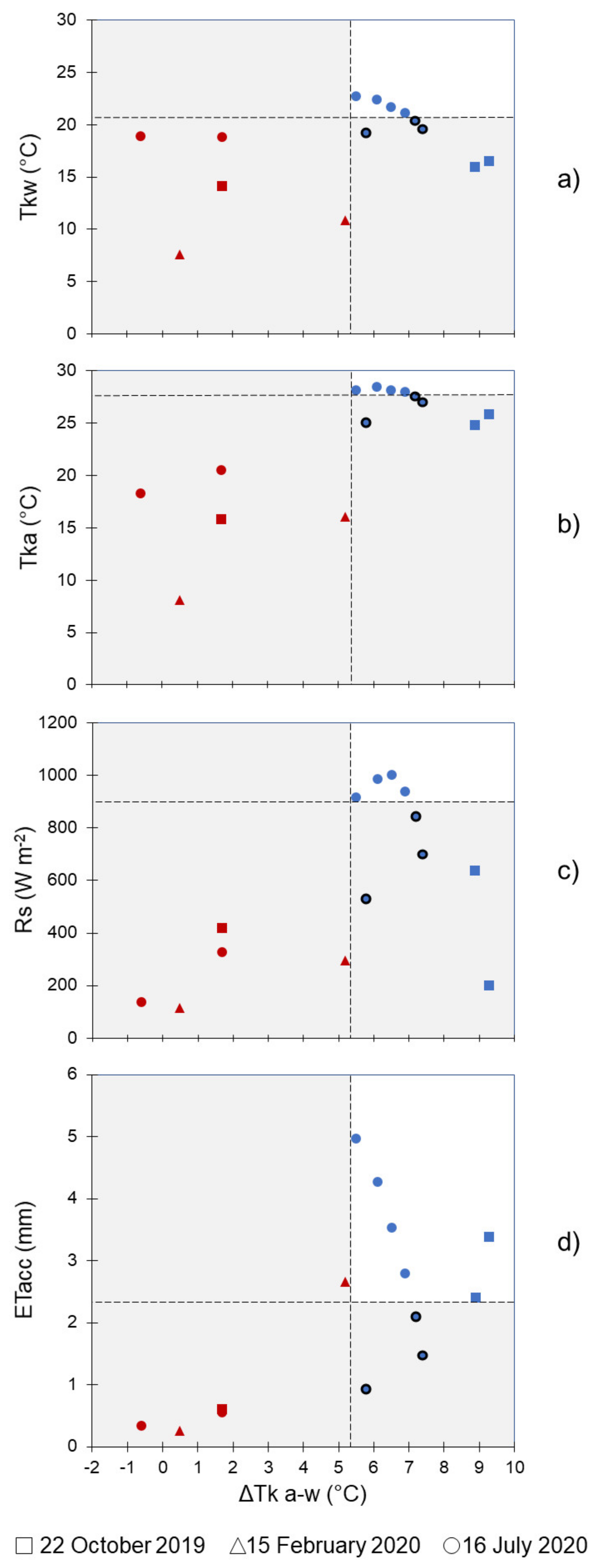
To summarize the reliability of the different experiments performed in this paper and to extrapolate general information about the conditions that ensure remote surveys without ambiguous detections, the two situations of (i) a possible overlapping of the WDN range with SDN and VDN ranges and (ii) a possible occurrence of false detections are represented in 2D graphs (Figure 7). The graphs consider both the thermal contrast between water and atmosphere (ΔTk a–w) and other measurable quantities, such as Tka, Tkw, solar radiation (Rs), and reference evapotranspiration accumulated during the focus day until the flight time (ETacc). While Tka, Tkw, and Rs provide information about the actual atmospheric conditions during the flight, ETacc is a proxy of the cumulative effects of surface–atmosphere interactions in the daylight hours prior to the flight.
Figure 7 identifies the flights with the WDN range overlapping to the SDN and VDN ranges with red symbols, while blue symbols are used for the remaining flights (the same information is provided in tabular form in the Supplementary Table S2). In all red flights, false water pixel detections occurred jointly with the observed overlapping of the DN ranges (Table 4), thereby implying that in those flights unambiguous detection of water presence was not possible. False detections occurred even in some blue flights. These are shown in the Figure as dots with a black contour. Therefore, optimal (i.e., with unambiguous detection) flights for the water presence identification using TIR images are represented as blue dots without any contour line (6 points out of 14).
Optimal flights were all characterized by high Tka, Tkw, and ΔTk a–w values, but high Tka, Tkw, and ΔTk a–w values did not always imply surveys with unambiguous detection. In particular, for Tka ≥ 24.8 °C and ΔTk a–w ≥ 5.5 °C only blue flights, with a different thermal response of water from other sources, were found. The afternoon flight in February 2020 occurred with ΔTk a–w = 5.2 °C, but with relatively low Tka (16 °C) and low radiation (Rs < 300 W m2). Among the blue flights, those producing false detections were three morning flights in July 2020, from 08:00 to 10:00. The last two flights occurred with ΔTk a–w > 7 °C and Rs ≥ 700 W m−2 (higher than the October 2019 flights); however, at that time of the day, the sunbeam was not yet able to sufficiently dry the bare soil surface and canopy (ETacc < 2.5 mm). On the other hand, the flight performed in October 2019 at 16:00 occurred with low radiation (Rs < 200 W m2), but at that time of the day significant evapotranspiration fluxes had already occurred (ETacc > 4.5 mm), resulting in the highest ΔTk a–w value (9.3 °C). Overall, in the analyzed case study, only a combined threshold of ΔTk a–w and ETacc (i.e., ΔTk a–w ≥ 5.5 °C and ETacc ≥ 2.4 mm) could detect all and only the blue uncontoured flights (Figure 7d).
The results shown in Figure 7 implicitly depend on the time of the day, i.e., on the time needed by vegetation cover and soil surface to dry. In both October 2019 and July 2020, when the air temperature was high enough, the thermal response of water in the afternoon was sufficiently different from other soil covers, even with low values of radiation (October 2019 at 16:00). On the other hand, with the temperatures observed in February, a survey performed at the end of daylight (15:30) with low Rs values did not provide satisfactory results, despite the relatively high ΔTk a–w and ETacc values. All surveys performed from late morning onwards with Tka ≥ 24.8 °C provided reliable results.
4. Discussion
In this contribution, we have proposed a method for the remote detection of water presence in river reaches based on combined TIR and RGB images, which requires the identification of suitable control matrices at the ground, representative of the water signature in the TIR band, for subsequent recognition of the wet river network in the whole surveyed area. Within the range of scenarios analyzed, we have demonstrated the validity of the method in warm and mid seasons, especially when the surveys were performed at times of the day when weather conditions allowed sufficient drying of the bare soil and vegetation. Furthermore, those surveys performed not too long after midday helped to minimize the shading effect [45]. Conversely, in the cold season survey, the methodology did not allow unambiguous recognition of the water pixels in either of the two flights carried out.
The main factor affecting reliable water pixel detection with TIR images is the difference between the temperatures of water and other typologies of surface objects targeted. The higher this difference, the higher the representativeness of the control matrices and the possibility that the thermal signatures of the different targets (in both the control matrices and the whole scene) do not overlap. Air temperature and, consequently, the thermal contrast between water and air are indicators of the magnitude of this difference. The results achieved in this study mostly depend on the significantly higher specific heat capacity of water as compared to bare soil (mainly sandy and sandy–pebbly material, in our case) and vegetation. When the land surface is sufficiently heated, the faster thermal response time of soil and vegetation allows clear detection of the colder water pixels.
The optimal timing of the surveys needs to be planned based on the expected variations in the thermal contrast between water and the surrounding landscape. These variations can be estimated using tools characterized by a different level of complexity. If the thermal features of the materials covering the surface are known (or hypothesized), a very detailed analysis could be achieved using land surface models (e.g., [46]), either in real–time or in forecast mode, to simulate surface temperatures of both water and other surface elements. Alternatively, as an intermediate level of detail, some weather variables could be monitored, like the air temperature and the stream temperature (if the latter is inspectable). Otherwise, as a rule of thumb, flights over Mediterranean catchments should be performed in the early afternoon (i.e., not too long after midday).
The operational hints are mainly valid for warm climates and need to be generalized for other climates where, for example, the water temperature can be higher than the surrounding surface for a great part of the day (e.g., frozen soils). Also, the actual reduction of informative content associated with false detections outside the geomorphic channels needs to be better addressed. In this study, false detections were used as an index of the reliability of the survey. However, the presence of many false water pixels might not represent an insurmountable problem. If the WDN range persists in the geomorphic channel, delineating the river network well, one can assume that the information provided by the UAV sensor is valid and useful, being possibly supported by RGB images. An example of that is provided by Figure 5c, where the water temperature is warmer than the soil and similar to vegetation. In that Figure, which can configure a typical situation of cold climates with ΔTk a–w = 0.5 °C, an accurate analysis of the combined RGB and thermal images not only allows one to infer water presence in the main channel but also the rivulet entering it. In future research, winter surveys should be increased and performed, differently from this study, also during hours of the day when the shading effect is minimized.
Support of RGB images becomes essential when surveys concern completely inaccessible areas. In these situations, remote visual inspection (i.e., using the visible band) of active river reaches not hidden by vegetation, if existing, is the only way to identify a suitable water control matrix in the corresponding TIR images. In such a context, every portion of the river network visible to the UAV sensors is a node to monitor. If the surveyed area is wide, making for a high probability of significant differences in flowing water temperatures along the stream, the water control matrices should be identified at regular distances, and the related WDN ranges should be considered as representative of well–defined subzones. The definition of the subzone extent depends on the thermal features of the water in the river network analyzed and needs further investigation.
Our experiments also provided other useful indications concerning the coupled use of UAVs and thermal sensors. Changes in the flight height did not produce a significant impact on the signal recorded by the thermal sensor. Indeed, the response of the thermal camera was similar regardless of the thickness of the atmospheric layer involved in the sensing procedure (Figure 3 and Table 4). The possibility of surveying objects at higher altitudes represents an important operational prospect since it allows the coverage of wider areas in less time. Conversely, the well–known problems induced by the use of an uncooled microbolometer thermal sensor occurred during several flights. The mounted microbolometer sensors are very sensitive to internal temperature variations [47,48] and are influenced by changing weather and climatic conditions, leading to inaccuracies in the measurements correlated to sensor noise. The thermal imaging camera in general produced less noise for intermediate air temperatures (roughly, between 18 and 25 °C, as the frequency distributions show). This disturbance did not lead to significant drawbacks during this application, in the light of the specific aims of the study. However, this would become a crucial issue if the objective were the exact measurement of the radiometric temperatures of the sensed objects [44,49]. In this case, a careful calibration of the TIR images with ground thermal references would be required for each type of target shot. Processing and interpreting TIR thermal images from UAVs are far from being straightforward [45,48,49,50,51,52,53]. The major issues associated with the processing of TIR images gathered via UAVs include shading effects and potential variations of weather conditions during the flight, which would vary the underlying thermal contrasts. While these problems are partially overcome by the proposed methodology, which considers only the relative difference in the thermal signature of the targeted objects, the presence of cooling systems in the thermal cameras mounted on UAVs would considerably increase the accuracy of surveys. This expected improvement, which nowadays has been mainly applied on systems operating in the mid–wave infrared (MWIR, i.e., approximately 3–5 μm) and requires high payloads (>2–3 kg), will be decisive in those cases with low thermal contrasts, making the proposed method more generally applicable, including to different climatic and environmental conditions.
5. Conclusions
In this study, we tested the efficiency of combined TIR and RGB images taken by drone to reliably detect the presence of water in a Mediterranean headwater catchment located in Southern Italy. Fourteen flights were performed at two different heights (22 m and 56 m) over a reach characterized by a permanent flow in three different periods, namely, October 2019, February 2020, and July 2020. The methodology consisted in taking TIR and RGB images simultaneously, using a double sensor camera (one thermal IR and one RGB) and analyzing raw data, without the need for detailed calibrations. For each image set, three “control matrices” representing water, vegetation, and bare soil thermal signatures were identified. For each control matrix, the minimum and maximum radiometric values were extracted, which were assumed as representative of the related cover type. The methodology allowed a correct detection of the water presence if applied to scenes characterized by an enhanced thermal contrast between flowing water and the surrounding environment. Our results also show that the difference between the thermal signature of water and other cover types was mainly related to the thermal contrast between water and air. Therefore, for a correct and unambiguous water pixel detection, sufficient drying of other cover types is needed, which is promoted by prolonged solar radiation and surface heating. As a result, late morning and early afternoon were the most suitable times to perform the surveys in autumn and summer. Conversely, the method failed in isolating the thermal signature of water in the surveys performed during winter, even though useful information could still be extracted from the related thermal images. In winter and all conditions with low thermal contrast, future research could move from using uncooled long–wave infrared (LWIR) sensors, such as those used in this research, to cooled MWIR sensors ensuring higher accuracy.
The proposed method represents a simple and effective alternative to existing methods for water detection. The main advantage of the proposed procedure is that it does not rely on any photogrammetric process, and it minimizes postprocessing efforts. The preliminary results discussed in this paper suggest a good potential of the tool for a range of important environmental applications, including the monitoring of the expansion and contraction dynamics of headwater stream networks.
Supplementary Materials
The following supporting information can be downloaded at: https://0-www-mdpi-com.brum.beds.ac.uk/article/10.3390/rs14010108/s1, Figure S1. (a) Three-dimensional representation of a high-resolution (20 cm) Lidar-derived digital terrain model of the study area (red borders). (b) Overlay of the study area on Lidar-derived high-resolution orthophoto. Elevation is represented by black contour lines. Figure S2. Surveys performed on 22 October 2019 at 09:15, 22 m flight altitude, the following images are shown: RGB image, with the delimitation of the geomorphic channel (a); the corresponding IR thermal image in false color, with the delimitation of the geomorphic channel (b); the pixels within the WDN range (c); the frequency distributions of the DN values of the thermal images, with three bands highlighting the WDN, SDN, and VDN ranges (d). Furthermore, information is provided about the date, time, and height of the flight; Tka, Tkw, and ΔTk a–w; and minimum and maximum values of the WDN, SDN, and VDN ranges. Figure S3. Surveys performed on 22 October 2019 at 12:45, 56 m flight altitude, the following images are shown: RGB image, with the delimitation of the geomorphic channel (a); the corresponding IR thermal image in false color, with the delimitation of the geomorphic channel (b); the pixels within the WDN range (c); the frequency distributions of the DN values of the thermal images, with three bands highlighting the WDN, SDN, and VDN ranges (d). Furthermore, information is provided about the date, time, and height of the flight; Tka, Tkw, and ΔTk a–w; and minimum and maximum values of the WDN, SDN, and VDN ranges. Figure S4. Surveys performed on 22 October 2019 at 16:00, 56 m flight altitude, the following images are shown: RGB image, with the delimitation of the geomorphic channel (a); the corresponding IR thermal image in false color, with the delimitation of the geomorphic channel (b); the pixels within the WDN range (c); the frequency distributions of the DN values of the thermal images, with three bands highlighting the WDN, SDN, and VDN ranges (d). Furthermore, information is provided about the date, time, and height of the flight; Tka, Tkw, and ΔTk a–w; and minimum and maximum values of the WDN, SDN, and VDN ranges. Figure S5. Surveys performed on 15 February 2020 at 07:30, 22 m flight altitude, the following images are shown: RGB image, with the delimitation of the geomorphic channel (a); the corresponding IR thermal image in false color, with the delimitation of the geomorphic channel (b); the pixels within the WDN range (c); the frequency distributions of the DN values of the thermal images, with three bands highlighting the WDN, SDN, and VDN ranges (d). Furthermore, information is provided about the date, time, and height of the flight; Tka, Tkw, and ΔTk a–w; and minimum and maximum values of the WDN, SDN, and VDN ranges. Figure S6. Surveys performed on 16 July 2020 at 06:00, 22 m and 56 m flight altitude, the following images are shown: RGB image, with the delimitation of the geomorphic channel (a,e); the corresponding IR thermal image in false color, with the delimitation of the geomorphic channel (b,f); the pixels within the WDN range (c,g); the frequency distributions of the DN values of the thermal images, with three bands highlighting the WDN, SDN, and VDN ranges (d,h). Furthermore, information is provided about the date, time, and height of the flight; Tka, Tkw, and ΔTk a–w; and minimum and maximum values of the WDN, SDN, and VDN ranges. Figure S7. Surveys performed on 16 July 2020 at 07:00, 56 m flight altitude, the following images are shown: RGB image, with the delimitation of the geomorphic channel (a); the corresponding IR thermal image in false color, with the delimitation of the geomorphic channel (b); the pixels within the WDN range (c); the frequency distributions of the DN values of the thermal images, with three bands highlighting the WDN, SDN, and VDN ranges (d). Furthermore, information is provided about the date, time, and height of the flight; Tka, Tkw, and ΔTk a–w; and minimum and maximum values of the WDN, SDN, and VDN ranges. Figure S8. Surveys performed on 16 July 2020 at 08:00, 22 m flight altitude, the following images are shown: RGB image, with the delimitation of the geomorphic channel (a); the corresponding IR thermal image in false color, with the delimitation of the geomorphic channel (b); the pixels within the WDN range (c); the frequency distributions of the DN values of the thermal images, with three bands highlighting the WDN, SDN, and VDN ranges (d). Furthermore, information is provided about the date, time, and height of the flight; Tka, Tkw, and ΔTk a–w; and minimum and maximum values of the WDN, SDN, and VDN ranges. Figure S9. Surveys performed on 16 July 2020 at 09:00, 22 m and 56 m flight altitude, the following images are shown: RGB image, with the delimitation of the geomorphic channel (a,e); the corresponding IR thermal image in false color, with the delimitation of the geomorphic channel (b,f); the pixels within the WDN range (c,g); the frequency distributions of the DN values of the thermal images, with three bands highlighting the WDN, SDN, and VDN ranges (d,h). Furthermore, information is provided about the date, time, and height of the flight; Tka, Tkw, and ΔTk a–w; and minimum and maximum values of the WDN, SDN, and VDN ranges. Figure S10. Surveys performed on 16 July 2020 at 11:00, 22 m and 56 m flight altitude, the following images are shown: RGB image, with the delimitation of the geomorphic channel (a,e); the corresponding IR thermal image in false color, with the delimitation of the geomorphic channel (b,f); the pixels within the WDN range (c,g); the frequency distributions of the DN values of the thermal images, with three bands highlighting the WDN, SDN, and VDN ranges (d,h). Furthermore, information is provided about the date, time, and height of the flight; Tka, Tkw, and ΔTk a–w; and minimum and maximum values of the WDN, SDN, and VDN ranges. Figure S11. Surveys performed on 16 July 2020 at 12:00, 22 m and 56 m flight altitude, the following images are shown: RGB image, with the delimitation of the geomorphic channel (a,e); the corresponding IR thermal image in false color, with the delimitation of the geomorphic channel (b,f); the pixels within the WDN range (c,g); the frequency distributions of the DN values of the thermal images, with three bands highlighting the WDN, SDN, and VDN ranges (d,h). Furthermore, information is provided about the date, time, and height of the flight; Tka, Tkw, and ΔTk a–w; and minimum and maximum values of the WDN, SDN, and VDN ranges. Figure S12. Surveys performed on 16 July 2020 at 13:00, 22 m and 56 m flight altitude, the following images are shown: RGB image, with the delimitation of the geomorphic channel (a,e); the corresponding IR thermal image in false color, with the delimitation of the geomorphic channel (b,f); the pixels within the WDN range (c,g); the frequency distributions of the DN values of the thermal images, with three bands highlighting the WDN, SDN, and VDN ranges (d,h). Furthermore, information is provided about the date, time, and height of the flight; Tka, Tkw, and ΔTk a–w; and minimum and maximum values of the WDN, SDN, and VDN ranges. Figure S13. Surveys performed on 16 July 2020 at 16:00, 22 m flight altitude, the following images are shown: RGB image, with the delimitation of the geomorphic channel (a); the corresponding IR thermal image in false color, with the delimitation of the geomorphic channel (b); the pixels within the WDN range (c); the frequency distributions of the DN values of the thermal images, with three bands highlighting the WDN, SDN, and VDN ranges (d). Furthermore, information is provided about the date, time, and height of the flight; Tka, Tkw, and ΔTk a–w; and minimum and maximum values of the WDN, SDN, and VDN ranges. Table S1. Weather conditions during flight days (data from the Fitterizzi weather station). Highlighted lines refer to the hours when the flights are performed. Table S2. Results Summary.
Author Contributions
Conceptualization, M.M., A.S., G.B. and G.M.; methodology, M.M. supported by A.S.; validation, M.M., A.S. and G.B.; formal analysis, M.M. and A.S.; investigation, M.M.; data curation, M.M.; writing–original draft preparation, M.M. and A.S., supported by G.B. and G.M.; writing–review and editing, A.S., supported by M.M., G.B. and G.M.; visualization, M.M. and A.S.; project administration, G.B.; funding acquisition, G.B. All authors have read and agreed to the published version of the manuscript.
Funding
This study was supported by the European Research Council (ERC) DyNET project funded through the European Community’s Horizon 2020–Excellent Science–Programme (grant agreement H2020–EU.1.1.–770999).
Data Availability Statement
Weather data are delivered, upon request, by the “Centro Funzionale Multirischi–ARPACAL” (http://www.cfd.calabria.it/, accessed on 3 November 2021). The other data presented in this study are available on request from the corresponding author.
Acknowledgments
The authors thank the “Centro Funzionale Multirischi” of the Calabrian Regional Agency for the Protection of the Environment for providing the observed meteorological dataset.
Conflicts of Interest
The authors declare no conflict of interest.
References
- Manfreda, S.; McCabe, M.F.; Miller, P.E.; Lucas, R.; Pajuelo Madrigal, V.; Mallinis, G.; Dor, E.B.; Helman, D.; Estes, L.; Ciraolo, G.; et al. On the use of unmanned aerial systems for environmental monitoring. Remote Sens. 2018, 10, 641. [Google Scholar] [CrossRef] [Green Version]
- Watts, A.C.; Ambrosia, V.G.; Hinkley, E.A. Unmanned aircraft systems in remote sensing and scientific research: Classification and considerations of use. Remote Sens. 2012, 4, 1671–1692. [Google Scholar] [CrossRef] [Green Version]
- Whitehead, K.; Hugenholtz, C.H. Remote sensing of the environment with small Unmanned Aircraft Systems (UASs), part 1: A review of progress and challenges. J. Unmanned Veh. Syst. 2014, 2, 69–85. [Google Scholar] [CrossRef]
- Whitehead, K.; Hugenholtz, C.H.; Myshak, S.; Brown, O.; LeClair, A.; Tamminga, A.; Barchyn, T.E.; Moorman, B.; Eaton, B. Remote sensing of the environment with small Unmanned Aircraft Systems (UASs), part 2: Scientific and commercial applications. J. Unmanned Veh. Syst. 2014, 2, 86–102. [Google Scholar] [CrossRef] [Green Version]
- Tomaštík, J.; Mokroš, M.; Surový, P.; Grznárová, A.; Merganič, J. UAV RTK/PPK Method–An optimal solution for mapping inaccessible forested areas? Remote Sens. 2019, 11, 721. [Google Scholar] [CrossRef] [Green Version]
- Turner, D.; Lucieer, A.; Watson, C. An Automated technique for generating georectified mosaics from ultra–high resolution Unmanned Aerial Vehicle (UAV) imagery, based on Structure from Motion (SfM) point clouds. Remote Sens. 2012, 4, 1392–1410. [Google Scholar] [CrossRef] [Green Version]
- Turner, D.; Lucieer, A.; Wallace, L. Direct georeferencing of ultrahigh–resolution UAV imagery. IEEE Trans. Geosci. Remote Sens. 2014, 52, 2738–2745. [Google Scholar] [CrossRef]
- DeBell, L.; Anderson, K.; Brazier, R.E.; King, N.; Jones, L. Water resource management at catchment scales using lightweight UAVs: Current capabilities and future perspectives. J. Unmanned Veh. Syst. 2015, 4, 7–30. [Google Scholar] [CrossRef]
- Jensen, A.M.; Neilson, B.T.; McKee, M.; Chen, Y. Thermal remote sensing with an autonomous unmanned aerial remote sensing platform for surface stream temperatures. In Proceedings of the 2012 IEEE International Geoscience and Remote Sensing Symposium, IEEE, Munich, Germany, 22–27 July 2012; pp. 5049–5052. [Google Scholar]
- Tamminga, A.; Hugenholtz, C.; Eaton, B.; Lapointe, M. Hyperspatial remote sensing of channel reach morphology and hydraulic fish habitat using an Unmanned Aerial Vehicle (UAV): A first assessment in the context of river research and management. River Res. Appl. 2015, 31, 379–391. [Google Scholar] [CrossRef]
- Woodget, A.S.; Carbonneau, P.E.; Visser, F.; Maddock, I.P. Quantifying submerged fluvial topography using hyperspatial resolution UAS imagery and structure from motion photogrammetry. Earth Surf. Process. Landf. 2015, 40, 47–64. [Google Scholar] [CrossRef] [Green Version]
- Spence, C.; Mengistu, S. Deployment of an unmanned aerial system to assist in mapping an intermittent stream. Hydrol. Process. 2016, 30, 493–500. [Google Scholar] [CrossRef]
- Pai, H.; Malenda, H.F.; Briggs, M.A.; Singha, K.; González–Pinzón, R.; Gooseff, M.N.; Tyler, S.W. Potential for small Unmanned Aircraft Systems applications for identifying groundwater–surface water exchange in a meandering river reach. Geophys. Res. Lett. 2017, 44, 11868–11877. [Google Scholar] [CrossRef] [Green Version]
- Woodget, A.S.; Austrums, R.; Maddock, I.P.; Habit, E. Drones and digital photogrammetry: From classifications to continuums for monitoring river habitat and hydromorphology. Wiley Interdiscip. Rev. Water 2017, 4, e1222. [Google Scholar] [CrossRef] [Green Version]
- Briggs, M.A.; Dawson, C.B.; Holmquist–Johnson, C.L.; Williams, K.H.; Lane, J.W. Efficient hydrogeological characterization of remote stream corridors using drones. Hydrol. Process. 2018, 33, 316–319. [Google Scholar] [CrossRef] [Green Version]
- Borg Galea, A.; Sadler, J.P.; Hannah, D.M.; Datry, T.; Dugdale, S.J. Mediterranean intermittent rivers and ephemeral streams: Challenges in monitoring complexity. Ecohydrology 2019, 12, e2149. [Google Scholar] [CrossRef]
- Casas–Mulet, R.; Pander, J.; Ryu, D.; Stewardson, M.J.; Geist, J. Unmanned Aerial Vehicle (UAV)–based Thermal Infra–Red (TIR) and optical imagery reveals multi–spatial scale controls of cold–water areas over a groundwater–dominated riverscape. Front. Environ. Sci. 2020, 8, 64. [Google Scholar] [CrossRef]
- Samboko, H.T.; Abas, I.; Luxemburg, W.M.J.; Savenije, H.H.G.; Makurira, H.; Banda, K.; Winsemius, H.C. Evaluation and improvement of remote sensing–based methods for river flow management. Phys. Chem. Earth, Parts A/B/C 2020, 117, 102839. [Google Scholar] [CrossRef]
- Kuhn, J.; Casas–Mulet, R.; Pander, J.; Geist, J. Assessing stream thermal heterogeneity and cold–water patches from UAV–based imagery: A matter of classification methods and metrics. Remote Sens. 2021, 13, 1379. [Google Scholar] [CrossRef]
- Datry, T.; Larned, S.T.; Tockner, K. Intermittent rivers: A challenge for freshwater ecology. Bioscience 2014, 64, 229–235. [Google Scholar] [CrossRef] [Green Version]
- Berger, E.; Haase, P.; Kuemmerlen, M.; Leps, M.; Schäfer, R.; Sundermann, A. Water quality variables and pollution sources shaping stream macroinvertebrate communities. Sci. Total. Environ. 2017, 587, 1–10. [Google Scholar] [CrossRef]
- Durighetto, N.; Vingiani, F.; Bertassello, L.E.; Camporese, M.; Botter, G. Intraseasonal drainage network dynamics in a headwater catchment of the Italian Alps. Water Resour. Res. 2020, 56, e2019WR025563. [Google Scholar] [CrossRef] [Green Version]
- Senatore, A.; Micieli, M.; Liotti, A.; Durighetto, N.; Mendicino, G.; Botter, G. Monitoring and Modeling drainage network contraction and dry down in Mediterranean headwater catchments. Water Resour. Res. 2021, 57, e2020WR028741. [Google Scholar] [CrossRef]
- Botter, G.; Vingiani, F.; Senatore, A.; Jensen, C.; Weiler, M.; McGuire, K.; Mendicino, G.; Durighetto, N. Hierarchical climate–driven dynamics of the active channel length in temporary streams. Sci. Rep. 2021, 11, 21503. [Google Scholar] [CrossRef]
- Rivas Casado, M.; Ballesteros Gonzalez, R.; Wright, R.; Bellamy, P. Quantifying the effect of aerial imagery resolution in automated hydromorphological river characterisation. Remote Sens. 2016, 8, 650. [Google Scholar] [CrossRef] [Green Version]
- McFeeters, S.K. The use of the Normalized Difference Water Index (NDWI) in the delineation of open water features. Int. J. Remote Sens. 1996, 17, 1425–1432. [Google Scholar] [CrossRef]
- Ouma, Y.O.; Tateishi, R. A water index for rapid mapping of shoreline changes of five East African Rift Valley lakes: An empirical analysis using Landsat TM and ETM+ data. Int. J. Remote Sens. 2006, 27, 3153–3181. [Google Scholar] [CrossRef]
- Du, Y.; Zhang, Y.; Ling, F.; Wang, Q.; Li, W.; Li, X. Water bodies’ mapping from Sentinel–2 imagery with modified Normalized Difference Water Index at 10–m spatial resolution produced by sharpening the SWIR band. Remote Sens. 2016, 8, 354. [Google Scholar] [CrossRef] [Green Version]
- Niroumand–Jadidi, M.; Vitti, A. Reconstruction of river boundaries at sub–pixel resolution: Estimation and spatial allocation of water fractions. ISPRS Int. J. Geo–Inf. 2017, 6, 383. [Google Scholar] [CrossRef] [Green Version]
- Li, L.; Yan, Z.; Shen, Q.; Cheng, G.; Gao, L.; Zhang, B. Water body extraction from very high spatial resolution remote sensing data based on fully convolutional networks. Remote Sens. 2019, 11, 1162. [Google Scholar] [CrossRef] [Green Version]
- Yang, X.; Li, Y.; Wei, Y.; Chen, Z.; Xie, P. Water body extraction from Sentinel–3 image with multiscale spatiotemporal super–resolution mapping. Water 2020, 12, 2605. [Google Scholar] [CrossRef]
- Bhaga, T.D.; Dube, T.; Shekede, M.D.; Shoko, C. Impacts of climate variability and drought on surface water resources in sub–saharan africa using remote sensing: A review. Remote Sens. 2020, 12, 4184. [Google Scholar] [CrossRef]
- Han, W.; Huang, C.; Duan, H.; Gu, J.; Hou, J. Lake phenology of freeze–thaw cycles using random forest: A case study of Qinghai Lake. Remote Sens. 2020, 12, 4098. [Google Scholar] [CrossRef]
- Wang, R.; Xia, H.; Qin, Y.; Niu, W.; Pan, L.; Li, R.; Zhao, X.; Bian, X.; Fu, P. Dynamic Monitoring of surface water area during 1989–2019 in the Hetao Plain using Landsat Data in Google Earth Engine. Water 2020, 12, 3010. [Google Scholar] [CrossRef]
- Kolli, M.K.; Opp, C.; Karthe, D.; Groll, M. Mapping of major land–use changes in the Kolleru Lake freshwater ecosystem by using Landsat Satellite images in Google Earth Engine. Water 2020, 12, 2493. [Google Scholar] [CrossRef]
- Jiang, Y.; Fu, P.; Weng, Q. Assessing the impacts of urbanization–associated land use/cover change on land surface temperature and surface moisture: A case study in the Midwestern United States. Remote Sens. 2015, 7, 4880–4898. [Google Scholar] [CrossRef] [Green Version]
- Xu, Y.; Wang, L.; Ross, K.W.; Liu, C.; Berry, K. Standardized soil moisture index for drought monitoring based on soil moisture active passive observations and 36 years of North American land data assimilation system data: A case study in the Southeast United States. Remote. Sens. 2018, 10, 301. [Google Scholar] [CrossRef] [Green Version]
- Gao, B.C. NDWI–A normalized difference water index for remote sensing of vegetation liquid water from space. Remote Sens. Environ. 1996, 58, 257–266. [Google Scholar] [CrossRef]
- Xu, H. Modification of Normalised Difference Water Index (NDWI) to enhance open water features in remotely sensed imagery. Int. J. Remote Sens. 2006, 27, 3025–3033. [Google Scholar] [CrossRef]
- Lacaux, J.P.; Tourre, Y.M.; Vignolles, C.; Ndione, J.A.; Lafaye, M. Classification of ponds from high–spatial resolution remote sensing: Application to Rift Valley Fever epidemics in Senegal. Remote Sens. Environ. 2007, 106, 66–74. [Google Scholar] [CrossRef]
- Ji, L.; Zhang, L.; Wylie, B. Analysis of dynamic thresholds for the Normalized Difference Water Index. Photogramm. Eng. Remote Sens. 2009, 75, 1307–1317. [Google Scholar] [CrossRef]
- Lillesand, T.; Kiefer, R.W.; Chipman, J. Remote Sensing and Image Interpretation, 7th ed.; John Wiley and Sons: New York, NY, USA, 2015. [Google Scholar]
- Handcock, R.N.; Torgersen, C.E.; Cherkauer, K.A.; Gillespie, A.R.; Tockner, K.; Faux, R.N.; Tan, J. Thermal Infrared Remote Sensing of Water Temperature in Riverine Landscapes. In Fluvial Remote Sensing for Science and Management; Carbonneau, P.E., Piégay, H., Eds.; Wiley–Blackwell: Chichester, UK, 2012; pp. 85–113. [Google Scholar]
- Dugdale, S.J.; Kelleher, C.A.; Malcolm, I.A.; Caldwell, S.; Hannah, D.M. Assessing the potential of drone–based thermal infrared imagery for quantifying river temperature heterogeneity. Hydrol. Process. 2019, 33, 1152–1163. [Google Scholar] [CrossRef]
- Dugdale, S.J.; Bergeron, N.E.; St–Hilaire, A. Spatial distribution of thermal refuges analysed in relation to riverscape hydromorphology using airborne thermal infrared imagery. Remote Sens. Environ. 2015, 160, 43–55. [Google Scholar] [CrossRef]
- Chen, F.; Dudhia, J. Coupling an advanced land surface–Hydrology model with the Penn State–NCAR MM5 modeling system. Part I: Model implementation and sensitivity. Mon. Weather Rev. 2001, 129, 569–585. [Google Scholar] [CrossRef] [Green Version]
- Olbrycht, R.; Więcek, B.; De Mey, G. Thermal drift compensation method for microbolometer thermal cameras. Appl. Opt. 2012, 51, 1788–1794. [Google Scholar] [CrossRef]
- Aragon, B.; Johansen, K.; Parkes, S.; Malbeteau, Y.; Al–Mashharawi, S.; Al–Amoudi, T.; Andrade, C.F.; Turner, D.; Lucieer, A.; McCabe, M.F. A calibration procedure for field and UAV–based uncooled thermal infrared instruments. Sensors 2020, 20, 3316. [Google Scholar] [CrossRef]
- Ribeiro–Gomes, K.; Hernández–López, D.; Ortega, J.F.; Ballesteros, R.; Poblete, T.; Moreno, M.A. Uncooled thermal camera calibration and optimization of the photogrammetry process for UAV applications in agriculture. Sensors 2017, 17, 2173. [Google Scholar] [CrossRef]
- Ebersole, J.L.; Liss, W.J.; Frissell, C.A. Cold water patches in warm streams: Physicochemical characteristics and the influence of shading. JAWRA J. Am. Water Resour. Assoc. 2003, 39, 355–368. [Google Scholar] [CrossRef]
- Harvey, M.C.; Rowland, J.V.; Luketina, K.M. Drone with thermal infrared camera provides high resolution georeferenced imagery of the Waikite geothermal area, New Zealand. J. Volcanol. Geotherm. Res. 2016, 325, 61–69. [Google Scholar] [CrossRef]
- Maes, W.H.; Huete, A.R.; Steppe, K. Optimizing the processing of UAV–based thermal imagery. Remote Sens. 2017, 9, 476. [Google Scholar] [CrossRef] [Green Version]
- Kelly, J.; Kljun, N.; Olsson, P.O.; Mihai, L.; Liljeblad, B.; Weslien, P.; Klemedtsson, L.; Eklundh, L. Challenges and best practices for deriving temperature data from an uncalibrated UAV thermal infrared camera. Remote Sens. 2019, 11, 567. [Google Scholar] [CrossRef] [Green Version]
Figure 1.
Subcatchment of the Turbolo creek closed at the Fitterizzi outlet. The red dot indicates the point where the surveys were carried out with the drone. In the RGB images taken at two different (winter and summer) dates, the geomorphic channel is delimited with yellow lines. The ford crosses the reach almost perpendicularly (tire tracks are visible in the images). The Fitterizzi gauge and weather station are indicated with a white dot.

Figure 2.
Some examples of the delimitation with polygons of the control matrix of water (yellow dots polygon), soil (red dashed polygon), and vegetation (yellow polygon) in three different survey days.
Figure 2.
Some examples of the delimitation with polygons of the control matrix of water (yellow dots polygon), soil (red dashed polygon), and vegetation (yellow polygon) in three different survey days.

Figure 3.
Time evolution of the DN ranges of the control matrices of water (WDN), soil (SDN), and vegetation (VDN) and observed kinetic temperatures of water (Tkw) and air (Tka) in the three survey days: 22 October 2019 (a), 15 February 2020 (b) and 16 July 2020 (c).
Figure 3.
Time evolution of the DN ranges of the control matrices of water (WDN), soil (SDN), and vegetation (VDN) and observed kinetic temperatures of water (Tkw) and air (Tka) in the three survey days: 22 October 2019 (a), 15 February 2020 (b) and 16 July 2020 (c).

Figure 4.
Surveys performed on 22 October 2019. For 09:15 (a–d), 12:45 (e–h), and 16:00 (i–l), the following images are shown: RGB image, with the delimitation of the geomorphic channel (a,e,i); the corresponding IR thermal image in false color, with the delimitation of the geomorphic channel (b,f,j); the pixels within the WDN range (c,g,k); the frequency distributions of the DN values of the thermal images, with three bands highlighting the WDN, SDN, and VDN ranges (d,h,l). Furthermore, information is provided about the date, time, and height of the flight; Tka, Tkw, and ΔTk a–w; and minimum and maximum values of the WDN, SDN, and VDN ranges. Images of all the flights performed during this day are provided in the Supplementary Materials.

Figure 5.
Surveys performed on 15 February 2020. At 07:30 (a–d), 15:30, 22 m flight altitude (e–h), and 15:30, 56 m flight altitude (i–l). For each row, the following images are shown: RGB image, with the delimitation of the geomorphic channel (a,e,i); the corresponding IR thermal image in false color, with the delimitation of the geomorphic channel (b,f,j); the pixels within the WDN range (c,g,k); the frequency distributions of the DN values of the thermal images, with three bands highlighting the WDN, SDN, and VDN ranges (d,h,l). Furthermore, information is provided about the date, time, and height of the flight; Tka, Tkw, and ΔTk a–w; and minimum and maximum values of the WDN, SDN, and VDN ranges.

Figure 6.
Surveys performed on 16 July 2020. At 07:00 (a–d), 08:00 (e–h), 10:00, 22 m (i–l), 56 m flight altitude (m–p), and 14:00 (q–t). For each row, the following images are shown: RGB image, with the delimitation of the geomorphic channel (a,e,i,m,q); the corresponding IR thermal image in false color, with the delimitation of the geomorphic channel (b,f,j,n,r); the pixels within the WDN range (c,g,k,o,s); the frequency distributions of the DN values of the thermal images, with three bands highlighting the WDN, SDN, and VDN ranges (d,h,lp,t). Furthermore, information is provided about the date, time, and height of the flight; Tka, Tkw and ΔTk a–w; and minimum and maximum values of WDN, SDN, and VDN ranges.

Figure 7.
For each of the 14 flights performed, several variables are shown against the thermal contrasts between water and air (ΔTk a–w): (a) kinetic temperature of air (Tka); (b) kinetic temperature of water (Tkw); (c) solar radiation (Rs); (d) accumulated evapotranspiration (ETacc). Red symbols represent the cases with overlapping of the WDN range with SDN and VDN ranges. Among the cases without overlapping (blue symbols), those where unambiguous detection of water presence was not possible are black contoured. The Figure shows one point for each date and time, despite the two different flight heights. In the only two cases in which the flights at 22 m and 56 m height provided different indications in Table 3 (i.e., 15 February 2020 at 15:30 and 16 July 2020 at 10:00), the worst condition was represented in the Figure (that is, 22 m and 56 m for the first and second date, respectively). The dashed lines divide the graphs so that the top right area (white background) includes the highest possible number of blue uncontoured symbols, based on the combined conditions ΔTk a–w > x and [Tka;Tkw;Rs;ETacc] > y, where x and y are selected threshold values.


Table 1.
Thermal and RGB sensors specification.
| Zenmuse XT2 | |
|---|---|
| Thermal sensor type | Uncooled VOx Microbolometer |
| Thermal sensor resolution | 640 × 512 pixels |
| Pixel pitch | 17 µm |
| Spectral band | 7.5–13.5 µm |
| Lens | 19 mm, FOV 32° × 26° |
| Camera visual sensor | CMOS, 1/1.7”, 4000 × 3000 pixels |
| Lens | 8 mm, FOV 57.12° × 42.44° |
Table 2.
Data surveys collection.
| Date | Number of Flights | CET/CEST Time | Flight Height (m) | GSD (cm) | RGB–IR Image Sets |
|---|---|---|---|---|---|
| 22 October 2019 1 | 3 | 09:15; 12:45; 16:00 | 6 | ||
| 15 February 2020 | 2 | 07:30; 15:30 | 22; 56 | 2; 5 | 4 |
| 16 July 2020 1 | 9 | 06:00–14:00 2 | 18 |
1 CEST time. 2 One flight every hour.
Table 3.
Water and air temperature measurements.
| Date | CET/CEST Time | Tkw (°C) | Tka (°C) | ΔTk a–w (°C) | ΔTkw 1 (°C) | Δtka 1 (°C) |
|---|---|---|---|---|---|---|
| 22 October 2019 | 09:15 | 14.1 | 15.8 | 1.7 | 2.4 | 10.0 |
| 12:45 | 15.9 | 24.8 | 8.9 | |||
| 16:00 | 16.5 | 25.8 | 9.3 | |||
| 15 February 2020 | 07:30 | 7.6 | 8.1 | 0.5 | 3.2 | 7.9 |
| 15:30 | 10.8 | 16 | 5.2 | |||
| 16 July 2020 | 06:00 | 18.9 | 18.3 | −0.6 | 3.9 | 10.2 |
| 07:00 | 18.8 | 20.5 | 1.7 | |||
| 08:00 | 19.2 | 25.0 | 5.8 | |||
| 09:00 | 19.6 | 27.0 | 7.4 | |||
| 10:00 | 20.4 | 27.6 | 7.2 | |||
| 11:00 | 21.1 | 28.0 | 6.9 | |||
| 12:00 | 21.7 | 28.2 | 6.5 | |||
| 13:00 | 22.4 | 28.5 | 6.1 | |||
| 14:00 | 22.7 | 28.2 | 5.5 |
1 maximum difference among all water (ΔTkw)/air (ΔTka) temperatures recorded during the drone flights in the date indicated.
Table 4.
Summary of the results concerning overlapping of WDN to VDN or SDN and true or false detection of water pixels outside the geomorphic channel. O: WDN overlapped; NO: WDN not overlapped. TD: true detection; FD: false detection. In some experiments both true and false water pixels were detected (TD–FD).
| Date | CET/CEST Time | WDN Overlapped with VDN and SDN | |
|---|---|---|---|
| 22 m Flight Height | 56 m Flight Height | ||
| 22 October 2019 | 09:15 | OTD–FD | OTD–FD |
| 12:45 | NOTD | NOTD | |
| 16:00 | NO | NO | |
| 15 February 2020 | 07:30 | OTD–FD | OTD–FD |
| 15:30 | OTD–FD | NOTD–FD | |
| 16 July 2020 | 06:00 | OTD–FD | OTD–FD |
| 07:00 | OTD–FD | OTD–FD | |
| 08:00 | NOTD–FD | NOTD–FD | |
| 09:00 | NOTD–FD | NOTD–FD | |
| 10:00 | NO | NOTD–FD | |
| 11:00 | NO | NO | |
| 12:00 | NO | NO | |
| 13:00 | NO | NO | |
| 14:00 | NO | NO | |
Publisher’s Note: MDPI stays neutral with regard to jurisdictional claims in published maps and institutional affiliations. |
© 2021 by the authors. Licensee MDPI, Basel, Switzerland. This article is an open access article distributed under the terms and conditions of the Creative Commons Attribution (CC BY) license (https://creativecommons.org/licenses/by/4.0/).
Share and Cite
MDPI and ACS Style
Micieli, M.; Botter, G.; Mendicino, G.; Senatore, A. UAV Thermal Images for Water Presence Detection in a Mediterranean Headwater Catchment. Remote Sens. 2022, 14, 108. https://0-doi-org.brum.beds.ac.uk/10.3390/rs14010108
AMA Style
Micieli M, Botter G, Mendicino G, Senatore A. UAV Thermal Images for Water Presence Detection in a Mediterranean Headwater Catchment. Remote Sensing. 2022; 14(1):108. https://0-doi-org.brum.beds.ac.uk/10.3390/rs14010108
Chicago/Turabian StyleMicieli, Massimo, Gianluca Botter, Giuseppe Mendicino, and Alfonso Senatore. 2022. "UAV Thermal Images for Water Presence Detection in a Mediterranean Headwater Catchment" Remote Sensing 14, no. 1: 108. https://0-doi-org.brum.beds.ac.uk/10.3390/rs14010108
Note that from the first issue of 2016, this journal uses article numbers instead of page numbers. See further details here.