Article

Estimation of Chlorophyll-a Concentrations in Small Water Bodies: Comparison of Fused Gaofen-6 and Sentinel-2 Sensors

Key Laboratory of Digital Earth Science, Aerospace Information Research Institute, Chinese Academy of Sciences, Beijing 100094, China
*
Author to whom correspondence should be addressed.
Submission received: 11 November 2021 / Revised: 29 December 2021 / Accepted: 30 December 2021 / Published: 5 January 2022
(This article belongs to the Special Issue Hyperspectral Remote Sensing Technology in Water Quality Evaluation)

Abstract

:
Chlorophyll-a concentrations in water bodies are one of the most important environmental evaluation indicators in monitoring the water environment. Small water bodies include headwater streams, springs, ditches, flushes, small lakes, and ponds, which represent important freshwater resources. However, the relatively narrow and fragmented nature of small water bodies makes it difficult to monitor chlorophyll-a via medium-resolution remote sensing. In the present study, we first fused Gaofen-6 (a new Chinese satellite) images to obtain 2 m resolution images with 8 bands, which was approved as a good data source for Chlorophyll-a monitoring in small water bodies as Sentinel-2. Further, we compared five semi-empirical and four machine learning models to estimate chlorophyll-a concentrations via simulated reflectance using fused Gaofen-6 and Sentinel-2 spectral response function. The results showed that the extreme gradient boosting tree model (one of the machine learning models) is the most accurate. The mean relative error (MRE) was 9.03%, and the root-mean-square error (RMSE) was 4.5 mg/m3 for the Sentinel-2 sensor, while for the fused Gaofen-6 image, MRE was 6.73%, and RMSE was 3.26 mg/m3. Thus, both fused Gaofen-6 and Sentinel-2 could estimate the chlorophyll-a concentrations in small water bodies. Since the fused Gaofen-6 exhibited a higher spatial resolution and Sentinel-2 exhibited a higher temporal resolution.

Graphical Abstract

1. Introduction

When monitoring water quality, chlorophyll-a (Chla) concentration plays a pivotal role and reflects the degree of eutrophication of water [1]. While using conventional means, the concentrations of Chla are manually measured in the field. This technique is costly and inefficient. In contrast, satellite remote sensing has a larger scope, presents data in real time, and has a low-cost performance compared to the conventional method.
Small water bodies, which represent important freshwater resources, include headwater streams, springs, ditches, flushes, small lakes, and ponds. The relatively narrow and fragmented nature of small water bodies makes monitoring Chla via most free remote sensors difficult. At present, the main remote sensing image data used for estimating Chla concentration include Coastal Zone Colour Scanner (CZCS) [2], Sea-viewing Wide Field Sensor (SeaWiFS) [3], Medium Resolution Imaging Spectrometer (MERIS) [4,5], Moderate Resolution Imaging Spectroradiometer (MODIS) [6,7,8], Visible Infrared Imaging Radiometer Suite (VIIRS) [9], Geostationary Ocean Colour Imager (GOCI) [10], Ocean and Land Colour Instrument (OLCI) [11,12], Second-Generation Global Imager aboard Global Change Observation Mission-Climate (SGLI/GCOM-C) [13,14,15], Landsat 8 OLI [16,17,18,19,20,21,22], Sentinel-2 MSI [17,23,24,25,26,27], Gaofen-1 Wide Field of View (WFV) [28], and HJ-1 [29]. Except for Sentinel-2, above mentioned free images have a spatial resolution bigger than 15 m, which are not very suitable for monitoring small water bodies. Sentinel-2 with a 10-m resolution is relatively suitable. In addition to the aforementioned publicly available data sets, there have been a few studies that have used commercial satellite data. For example, researchers have used Worldview-2 [30] to study Chla concentration in lakes and reservoirs, Geoeye [31] and SOPT [32] satellites to study the transparency of lakes and reservoirs, and PlanetScopte satellites [33] to monitor water quality in rivers.
Small water bodies Chla monitoring requires high spectral resolution. The characteristic absorption bands of chlorophyll a are 440 nm and 670 nm, and many models for satellite estimation of Chla often make use of these two characteristic bands. Since these 2 absorption bands are relatively narrow, broad-band satellites often fail to capture the feature, making Chla estimates less accurate. Most current research around Chla estimation focuses on satellites with chlorophyll signature bands, such as the water-color satellite SeaWiFS and the land satellite Sentinel-2.
Gaofen-6, a new satellite with a Pan-Multispectral Sensor (PMS) and wide field of view (WFV), was successfully launched on 2 June 2018. Gaofen-6 PMS can provide a 2 m panchromatic image and an 8 m multi-spectral image with four bands (including blue, green, red, and near-infrared bands). The orbit of the Gaofen-6 satellite is not fixed. Additionally, Gaofen-6 WFV has eight bands (including aerosol, blue, green, yellow, red, red-edge I, red-edge II, and near-infrared (NIR)) with a spatial resolution of 16 m. Gaofen-6 WFV has “red edge” spectral characteristics, which is crucial for Chla monitoring.
The existing models used to estimate Chla concentration mainly include empirical models [34,35], semi-analytical models [36,37], analytical models [38,39], water classification models [40,41], and machine learning (deep learning) models [19,42,43,44,45,46,47,48,49]. The empirical model uses the basic principle of the inherent optical parameters and provides the theoretical basis of the empirical algorithm; the semi-analytical method is based on the theory of radiation transmission of light underwater and constructs the relationship between the inherent optical parameters and the apparent optical parameters to estimate the Chla concentrations in water; the analytical method is based on the mechanism of optical radiation transmission in water, and it mainly uses the relationship between the components of the water body and the inherent optical parameters. The water classification models are based on water body classification, which mainly reflects the use of different models for estimating Chla concentrations in various water body categories. Machine learning and deep learning are involved in all engineering fields owing to the increase in computing power. Several studies have reported remote sensing estimation of water quality parameter inversion.
In summary, small water bodies Chla monitoring requires high spatial resolution and high spectral resolution. Therefore, fusing data from Gaofen-6 provides suitable resources for monitoring Chla in small water bodies similar to Sentinel-2. Figure 1 illustrates the technical roadmap of the present study. We will first fuse Gaofen-6 images using Gaofen-6 PMS and Gaofen-6 WFV images to obtain images with the 2 m resolution, eight spectral bands, and 90 km swath width. Secondly, we will compare five semi-empirical models and four machine learning models via simulated reflectance using fused Gaofen-6 and Sentinel-2 spectral response functions. Thirdly, we will choose the best model and apply it in Gaofen-6 and Sentinel-2 images to estimate Chla of the same small water bodies. At last, we will compare the obtained results between fused Gaofen-6 and Sentinel-2.

2. Materials and Methods

2.1. Materials

2.1.1. Study Area

Beijing’s latitude and longitude ranging from 115.7°E to 117.4°E, and 39.4°N to 41.6°N were considered as the study areas. These areas comprise five main water systems: the Jima River, Yongding River, North Canal, Chaobai River, Ji Canal, and four artificial reservoirs with water storage functions, namely, the Miyun Reservoir, Guanting Reservoir, Huairou reservoir, and Haizi Reservoir. The sampling sites of the in situ data in this study were distributed in the Summer Palace pond (Figure 2A), Beihai Park pond (Figure 2B), Grand Canal (Figure 2C), Guanting Reservoir (Figure 2D), Purple Bamboo Park pond (Figure 2E), and Yuyuantan Park pond (Figure 2F). The Summer Palace, Beihai Park, Purple Bamboo Park, and Yuyuantan Park are important tourism resources, and the water quality is indicative of the city’s maintenance of water bodies. The Guanting Reservoir exerts unlimited power during flood control, comprehensive management, and ecological restoration of the Yongding River. The location of the study area and the spatial distribution of Beijing’s built-up areas are illustrated in Figure 2.

2.1.2. Field Measurements

We measured and collected remote sensing reflectance (Rrs, sr−1) and samples points of the water body at the Guanting Reservoir, Yuyuantan Park, Summer Palace Park, Beihai Park, Grand Canal, and Purple Bamboo Park on 8 September 2016, 21 August 2019, 16 September 2019, 18 September 2019, 15 October 2019, and 25 October 2019, respectively; thereafter, we acquired 82 water body spectra in six field surveys (Table 1). The spectral type average is as shown in Figure 3a. For each field survey, we used GPS to record the latitude and longitude information and collected 1.5–2 L water samples from the water surface; these samples were sent to the laboratory to measure and analyze the Chla concentration. We collected surface water samples from the field and placed them in a low-temperature water sample box to minimize the potential changes brought about during transportation to the laboratory.
The satellite-to-ground synchronization experiment was set up on 18 September 2019 and 25 October 2019. The synchronized Gaofen-6 images corresponded to the Beihai Park field and Purple Bamboo Park field experiments conducted in the study area on 18 September and 25 October 2019, respectively. Information regarding the imaging time of the remote sensing images used, among other aspects, is given in Table 2.

2.1.3. Radiometric Measurements

The field experiments mainly comprised water body spectral measurements and simultaneous water body sampling. Spectral data were measured using an analytical spectral device (FieldSpec4 geophysical spectrometer Hi-Res NG) manufactured in the USA. This device allows continuous measurements in the 350–2500 nm wavelength range. In this study, the remote sensing reflectance of each in situ point was collected using the NASA ocean optics specification and the above-water surface method proposed by Tang et al. [50,51].
R r s λ = L u λ r s k y λ L s k y λ L p λ π / ρ p λ
where L u λ is the total upwelling spectral radiance above the water surface, r s k y λ L s k y λ is the direct upwelling radiance reflected on the water surface contributed by the sky, r s k y λ and calculated using the Fresnel formula,   L p λ is the simultaneously observed radiance of the reference panel, which has an accurately calibrated reflectance, and ρ p λ is the reflectance of the reference panel, which represents approximately 30%.

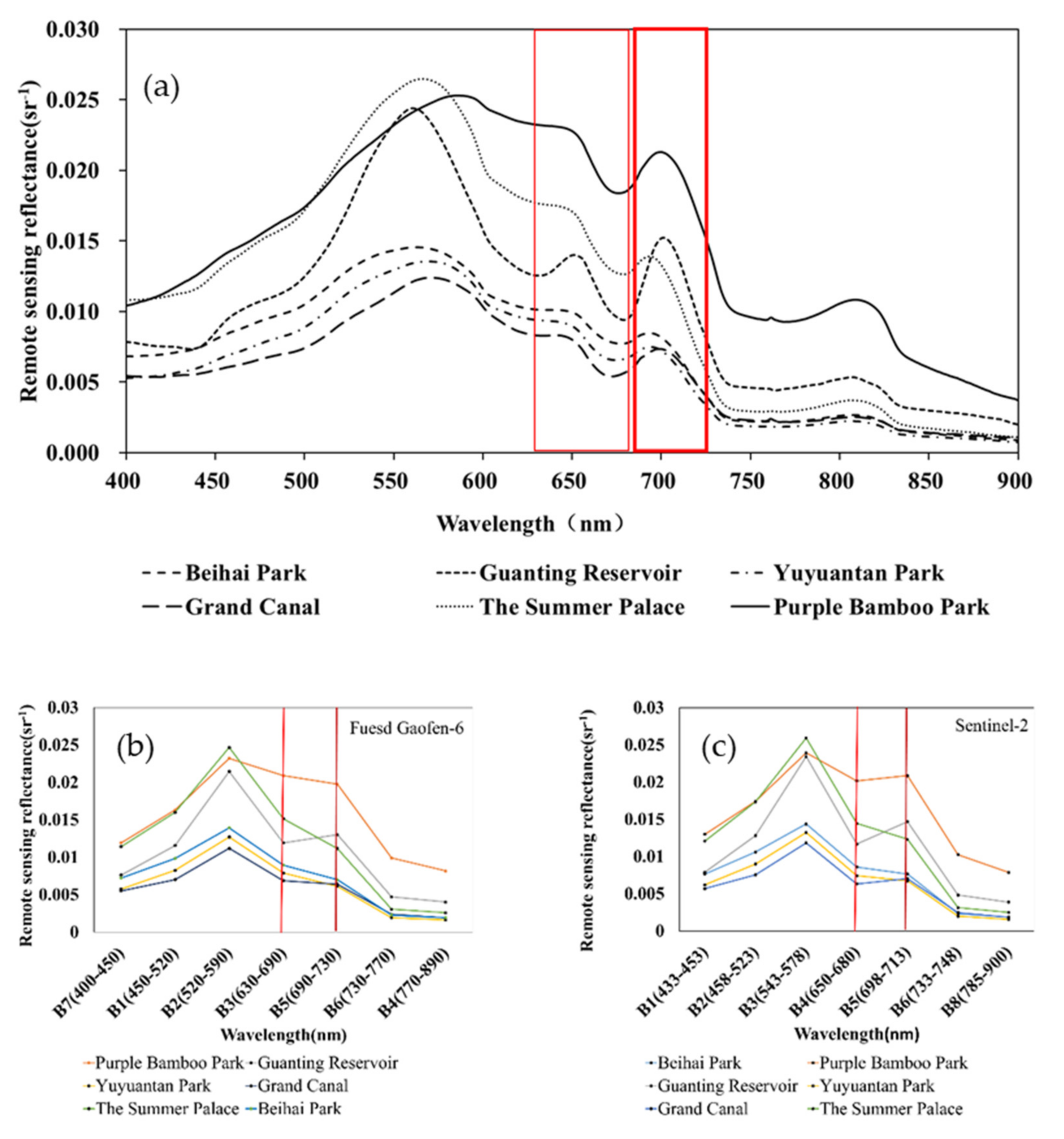
2.1.4. Bands Spectral Simulation

Because the in situ spectral data are spaced at 1 nm, and as the Gaofen-6 or Sentinel-2 satellites act as discrete spectral bands, each band has a certain width of wavelength response. To apply the in situ remote sensing reflectance to the Gaofen-6 and Sentinel-2 images, it is necessary to simulate the reflectance to the multi-spectral satellite band simulation reflectance via Equation (2) [7]:
R r s λ i = λ m i n λ m a x R r s λ f λ d λ λ m i n λ m a x f λ d λ
where f(λ) is the relative spectral response function of the Gaofen-6 and Sentinel-2 bands, and λ m a x and λ m i n are the wavelength ranges of the spectral response function.
In situ spectra from different in situ samples at the same site are small variations, we enhanced the information on absorption valleys and reflection peaks of in situ spectra with Chla concentrations, we have averaged the spectra from the same site in Figure 3. Figure 3 presents the mean spectra values of our collection study areas, and we discovered that Chla-associated spectral were present in all of these study areas. The absorption valleys and reflection peaks at 675 and 705 nm (Figure 3) were preserved following bandwidth averaging. Furthermore, the two vertical red lines in Figure 3 indicate that the 675 nm and 705 nm features were retained; therefore, the absorption valleys and reflection peaks can be applied to Gaofen-6 and Sentinel-2 images spectrum.

2.1.5. Chlorophyll-a Concentrations Measurement

The water samples were first filtered using Whatman GF/F fiberglass filters and then frozen at −20 °C for 24 h. The filter membranes were soaked in anhydrous ethanol at a temperature of 85 °C and a concentration of 90%, and the test tubes with hot ethanol (together with a special test tube holder) were quickly placed in a thermostatic water bath at 85 °C for 2 min; after acidification with 1 mol/L hydrochloric acid, the absorbance was measured at 665 and 750 nm using a UV2550 spectrophotometer, and the Chla concentrations were determined [52].

2.2. Remote Sensing Materials

In this study, Gaofen-6 and Sentinel-2 remote sensing images were used. The Gaofen-6 PMS has a spatial resolution of 2 m of the panchromatic band, while the four bands (blue, green, red, and NIR) have a spatial resolution of 8 m. The Gaofen-6 WFV has eight bands (aerosol, blue, green, yellow, red, red-edge I, red-edge II, and NIR) with a spatial resolution of 16 m and a wavelength of 0.45–0.9 nm. Information on Gaofen-6 is available at http://36.112.130.153:7777/DSSPlatform/productSearch.html (accessed on 25 October 2021). Sentinel-2 has 13 bands (aerosol, blue, green, red, red-edge I, red-edge II, red-edge III, NIR, narrow-edge near-infrared, water vapor, short-wave infrared cirrus band, short-wave infrared I, short-wave infrared II), with a wavelength range of 0.43–2.19 nm. Information on Sentinel-2 is available at https://scihub.copernicus.eu/dhus/#/home (accessed on 25 October 2021). Certain bands in Gaofen-6 and Sentinel-2 are remarkably similar (Table 3).
For the fused Gaofen-6, there are the main three steps of image processing: image fusion as well as geometric and atmospheric corrections. The image processing proceeded as illustrated in Figure 4. We first used image fusion to obtain a fused Gaofen-6 with a spatial resolution of 2 m and a spectral resolution of eight bands; then, we performed a geometric correction of the fused Gaofen-6 and Sentinel-2 for a comparative analysis of the two; and finally, we performed an atmospheric correction to complete the pre-processing of the fused Gaofen-6.

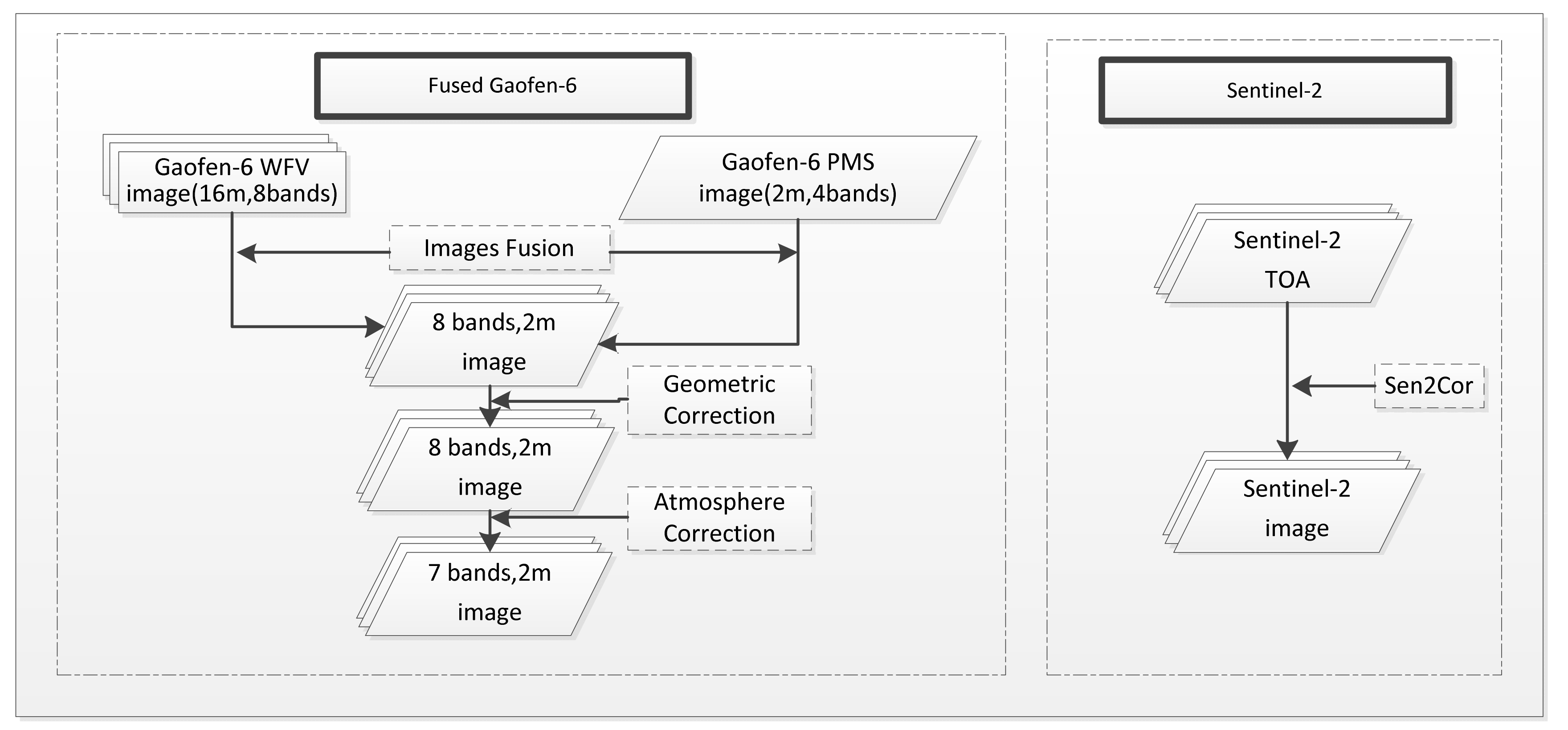
2.2.1. Fused Gaofen-6 Remote Sensing Materials

For fused Gaofen-6 images, image fusion uses pixel-knife software [53], a fusion algorithm provided by the software. We corrected the misalignment between bands using a fine alignment algorithm with gradient tracking to ensure that the inter-band alignment error is less than 0.1 image element. Afterwards, we fused the PAN and MSS images using an optimal model fusion algorithm based on multi-conditional constraints. This approach ensures that the spectral shape and the value of the fusion remain essentially unchanged.
For fused Gaofen-6 images, geometric corrections were made using Long’s method [54], which aims to provide geometric correction accuracy at the sub-meter level. Moreover, high-resolution satellites reveal certain geometric distortions that need to be eliminated. The reference image is the Google Online Satellite Image, which includes remote sensing data on all Google platforms from 0.5–200 m. Automatically extracts the geometric control points in the image, extracts the connection point in the block overlap area, uses Shuttle Radar Topography Mission Digital Elevation Model (STRM DEM) assistance to perform the regional network adjustment, and reason for all partition images multi-class coefficient model is correct, and finally subunit the image to splicing the full geometric refinement image [54]. The geometric precision correction represents the key step of atmospheric correction pre-processing in this study.
For the fused Gaofen-6 atmospheric correction of water bodies, we used the Relative Radiation Normalization [55] method since the atmospheric correction of small turbid water bodies requires short-wave infrared correction of aerosol information. However, because fused Gaofen-6 does not set the corresponding band, we could not use the traditional water body atmospheric correction method., we can use the same area’s Sentinel-2 as reference images to complete the Fused Gaofen-6’s Atmospheric correction., and by finding the radiation invariant control points for band-by-band atmospheric correction after geometric precision correction. In this study, Sentinel-2 is the reference image that can be used for the atmospheric correction of fused Gaofen-6. Before atmospheric correction is performed, the remote sensing data from both sources must be processed at identical resolution. Therefore, we resampled all bands of Sentinel-2 to 10 m using the Sentinel application platform medium and high-resolution plug [56] while the fused Gaofen-6 bands were resampled at a 10 m resolution using the down-sampling method. The atmospheric correction method is crucial in finding the radiometric control point, and we used an iteratively re-weighted multivariate alteration detection method [55] to identify it. The procedural steps involve correcting and referencing the image according to the characteristics of different typical variables to obtain the MAD and allow multiple iterations. If its feature value satisfies the chi-square distribution [55] and the threshold is greater than 0.95, it is considered a radiometric control point. The atmospheric correction of the water body can be completed by regressing the reflectance from Sentinel-2 and the DN values from fused Gaofen-6 using the radiometric control point. The relative radiation normalization method for atmospheric correction requires the reference and sample images to be corrected to the same band settings and similar spectral response functions. By comparing the simulated bands, the Gaofen-6 and Sentinel-2 were in good agreement with the spectral information of the same bands (Figure 5a). Thus, the fused Gaofen-6 can be atmosphere corrected using the relative radiation normalization method. The atmospheric correction using relative radiometric normalization is basically around the 1:1 line, which can accurately estimate the Chla concentration. The randomly selected pixel value of 3 × 3 of the water body in the Sentinel-2 image as a blended image element includes the outliers indicated in Figure 5b.
Sentinel-2 bands do not include the yellow band; hence, fused Gaofen-6 following atmospheric correction has only seven bands: blue (450–520 nm), green (520–590 nm), red (630–690 nm), NIR (770–890 nm), red-Edge (690–730 nm), red-Edge II (730–770 nm), and coastal aerosol (400–450 nm).

2.2.2. Sentinel-2 Remote Sensing Materials

For Sentinel-2 images, the only pre-processing step was atmospheric correction. We have access to the Top of Atmosphere Reflectance (TOA) level dataset at the official website, and we used the Sen2Cor plug-in for atmospheric correction to obtain the reflectance level dataset.

2.3. Accuracy Evaluation

Accuracy evaluation was performed using the mean relative error (MRE) and root mean square error (RMSE) with the following formulas:
M R E = 1 n 1 n R i R j R j × 100 %
R M S E = 1 n R i R j 2 n
where n stands for the number of points in this study, Ri represents the estimated Chla concentration value, and Rj represents the in situ Chla concentration.

2.4. Methods

We compared the accuracy of a semi-empirical model to a machine learning model for estimating Chla concentration. First, to determine the division of the dataset, the semi-empirical model dataset is mainly divided into two parts: the modeling dataset and the validation dataset (SE-V). The machine learning model dataset was divided into three main parts: the training dataset, the validation dataset, and the test dataset (ML-T). For comparisons, we divided the dataset at a 9 (N = 74):1 (M = 8) ratio and verified the robustness of the different models by sequentially sampling eight points as the SE-V and the ML-T. We used 74 points to train the semi-empirical model and the machine learning model using a 5K fold division into a training set and a validation set.
For the semi-empirical model, the independent variables included two forms of Rrs (675 nm)/Rrs (705 nm) and Rrs (705 nm))/Rrs (675 nm). Based on the correlation between the above two forms and the concentration of Chla, and chose Rrs (675 nm)/Rrs(705 nm) as the independent variable factor. Chla exhibited strong absorption characteristics at 675 nm; thus, the reflectance at 675 nm revealed an obvious trough, and the ratio of 675 nm/705 nm can be used to estimate the inverse Chla concentrations [3]. Simultaneously, five functional forms were proposed for comparison: linear, exponential, logarithmic, power, and quadratic functions [34]. The fitting results of the five models were compared, and the optimal model was selected (Table 4). We used the accuracy evaluation indexes MRE and RMSE for comparing the simulated spectrum estimate Chla concentrations with the measured Chla concentrations to check the model accuracy.
For the machine learning model, the machine learning model is estimated based on the non-linear fitting relationship between remote sensing reflectance and Chla concentrations in water bodies; moreover, multiple linear regression (LR), multiple Bayesian regression (BR), extreme gradient boosting tree (BST), and artificial neural networks (ANN) were used in this study. LR assigns all inputs to a regression coefficient, the loss function is used, and the least-squares method is solved. BR assigns all inputs to a regression coefficient, and the loss function adds regularisation and uses the least-squares method to solve. BST predicts multiple weak classifiers superimposed on a final model. ANN is a model prediction that uses multiple layers of neurons and uses a combination of activation functions.
The input feature of the machine learning model is important. We focused on the band selected as the input. According to Section 2.2.1, seven bands were left in the fused Gaofen-6 images after atmospheric correction. We tested five combinations: (1) six bands without the red-edge band; (2) total seven bands; (3) eight inputs_1, including seven bands, the ratio of the red-edge band to the red band; (4) eight inputs_2, including seven bands, the ratio of the red band to the red-edge band; (5) nine inputs, including seven bands, the ratio of the red-edge band to the red band, and the ratio of the red band to the red-edge band.
The MRE of six inputs, seven inputs, eight inputs_1, eight inputs_2 and nine inputs were 12.22%, 12.52%,21.24%,16.5% and 7.9%, respectively, and the RMSEs were 3.55 mg/m3, 3.84 mg/m3, 4.49 mg/m3, 3.7 mg/m3 and 1.72 mg/m3, respectively. It was found that nine inputs (seven reflectance bands, two bands of red-edge band, and ratio of red band) worked best in the validation set; therefore, multiple regression input using nine inputs [19] was used to estimate the Chla concentration (Figure 6). The selection of the characteristic band showed that using the Rrs (675 nm)/Rrs (705 nm) ratio in the characteristic band resulted in a remarkably smaller error and further showed a strong correlation between Rrs (675 nm)/Rrs (705 nm) and Chla concentrations.

3. Results

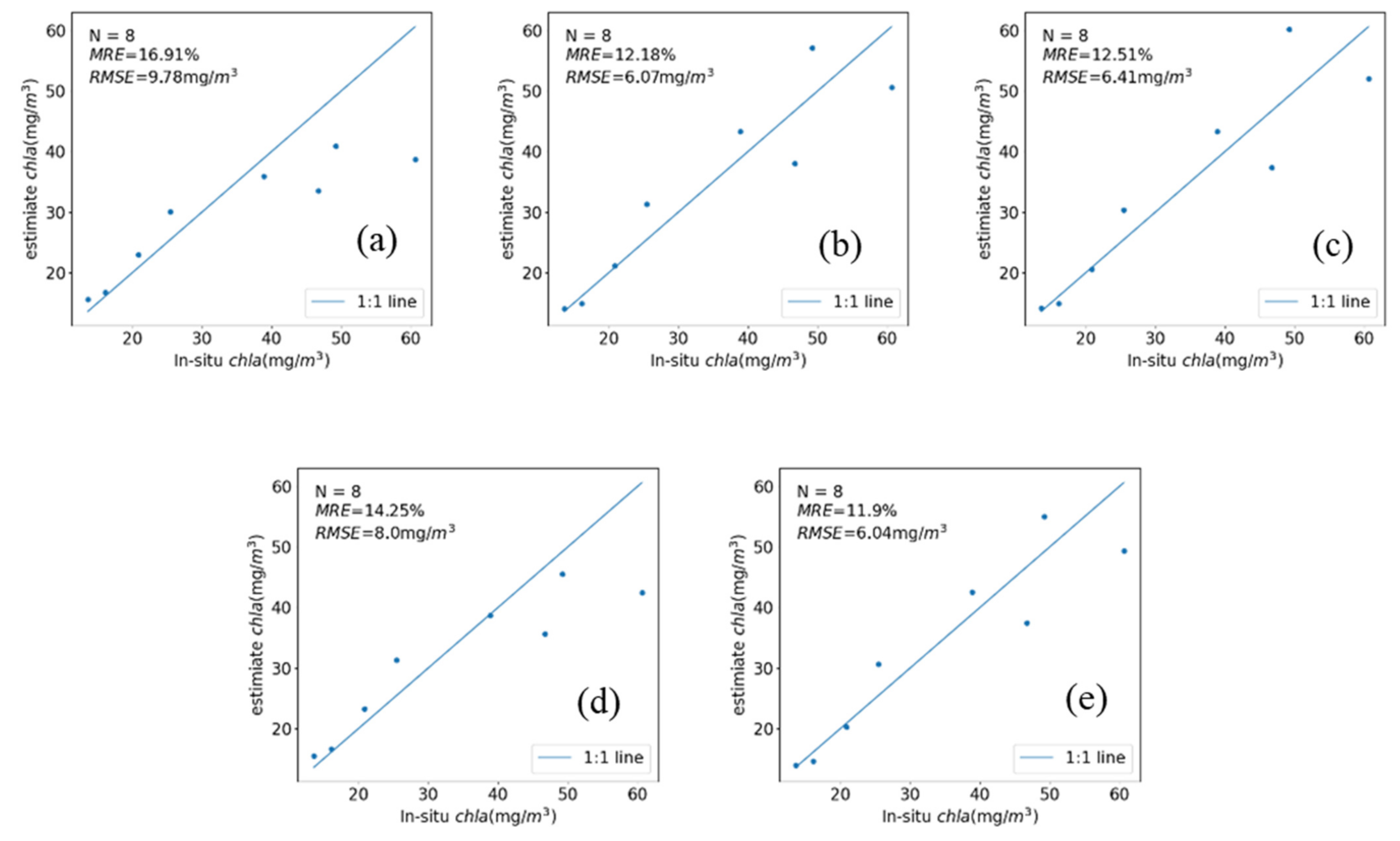
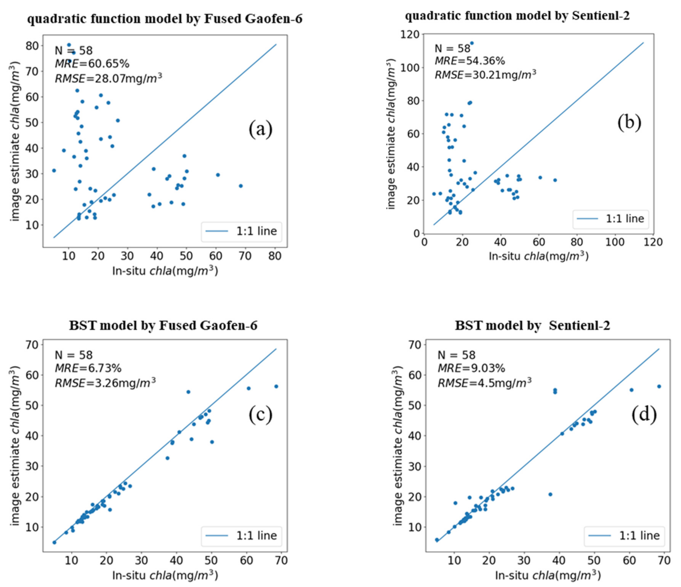
3.1. Semi-Empirical Model

3.1.1. Fused Gaofen-6 Semi-Empirical Model

For fused Gaofen-6, we listed the formulas for the five models (Table 5). The verification diagram (Figure 7) reveals that the quadratic function model is the best among the five models [34].
Based on the verification analysis, the linear and logarithmic models exhibit a low potential >40 mg/m3, power function, and quadratic function model distribution around the 1:1 line; however, the quadratic function model exhibits the lowest MRE and RMSE, attaining 11.9%, 6.04 mg/m3.

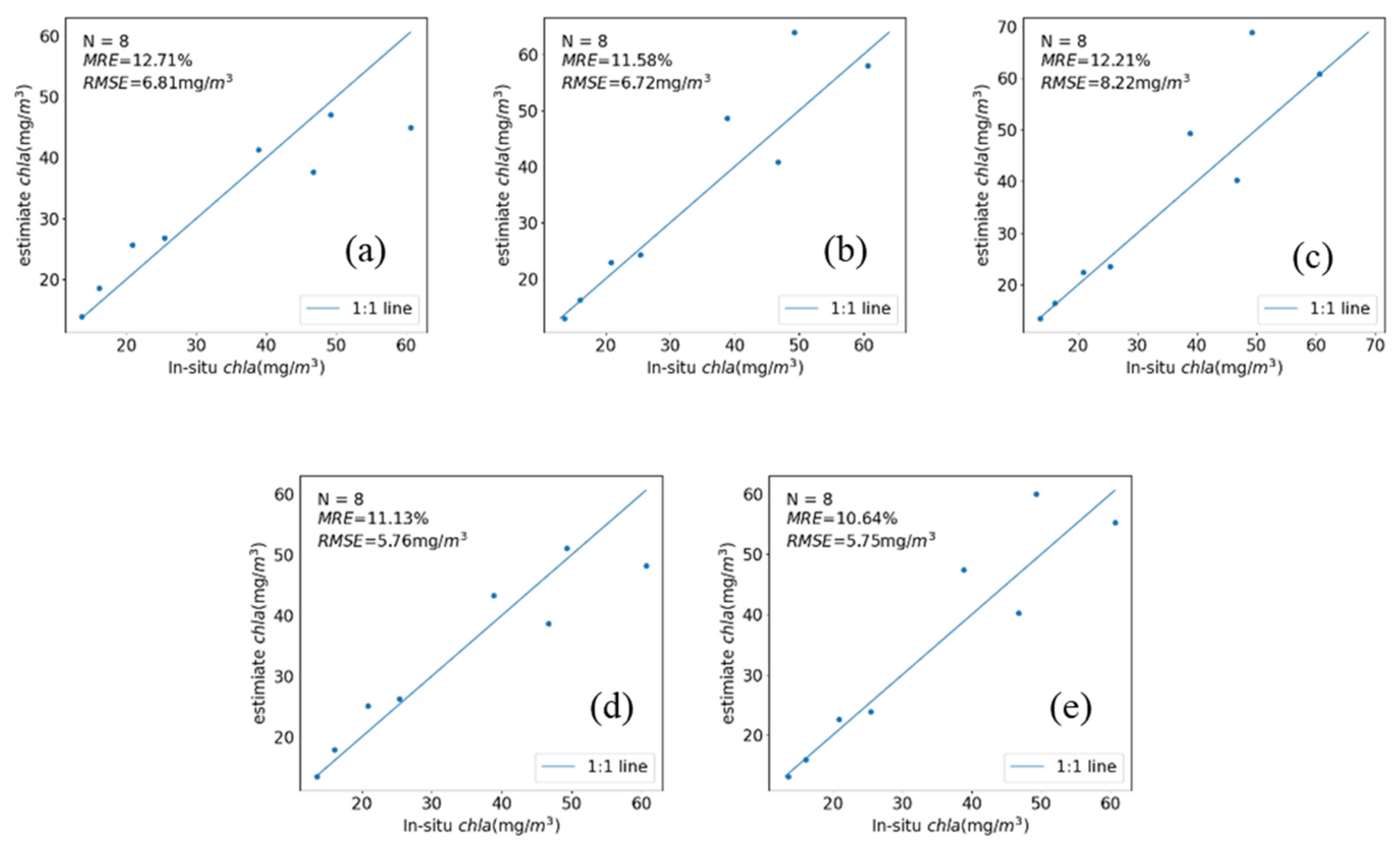
3.1.2. Sentinel-2 Semi-Empirical Model

For Sentinel-2, we listed the formulas for the five models (Table 6); according to the verification diagram (Figure 8), the quadratic function model is the best among these five models.
Based on the verification analysis, the linear model reveals low exponential model, power function, logarithmic model, and quadratic function model distributed around the 1:1 line >45 mg/m3; however, the quadratic function model exhibits the lowest MRE of 10.64% and RMSE of 5.75 mg/m3.
Among the semi-analytical models, either fused Gaofen-6 or Sentinel-2, the quadratic function model showed the best fit; thus, we determined that the quadratic function model is the most suitable semi-analytical model for estimating Chla concentrations in small water bodies. We compared the accuracy of the traditional algorithmic model with that of the quadratic function model (Appendix A Table A1 and Table A2).

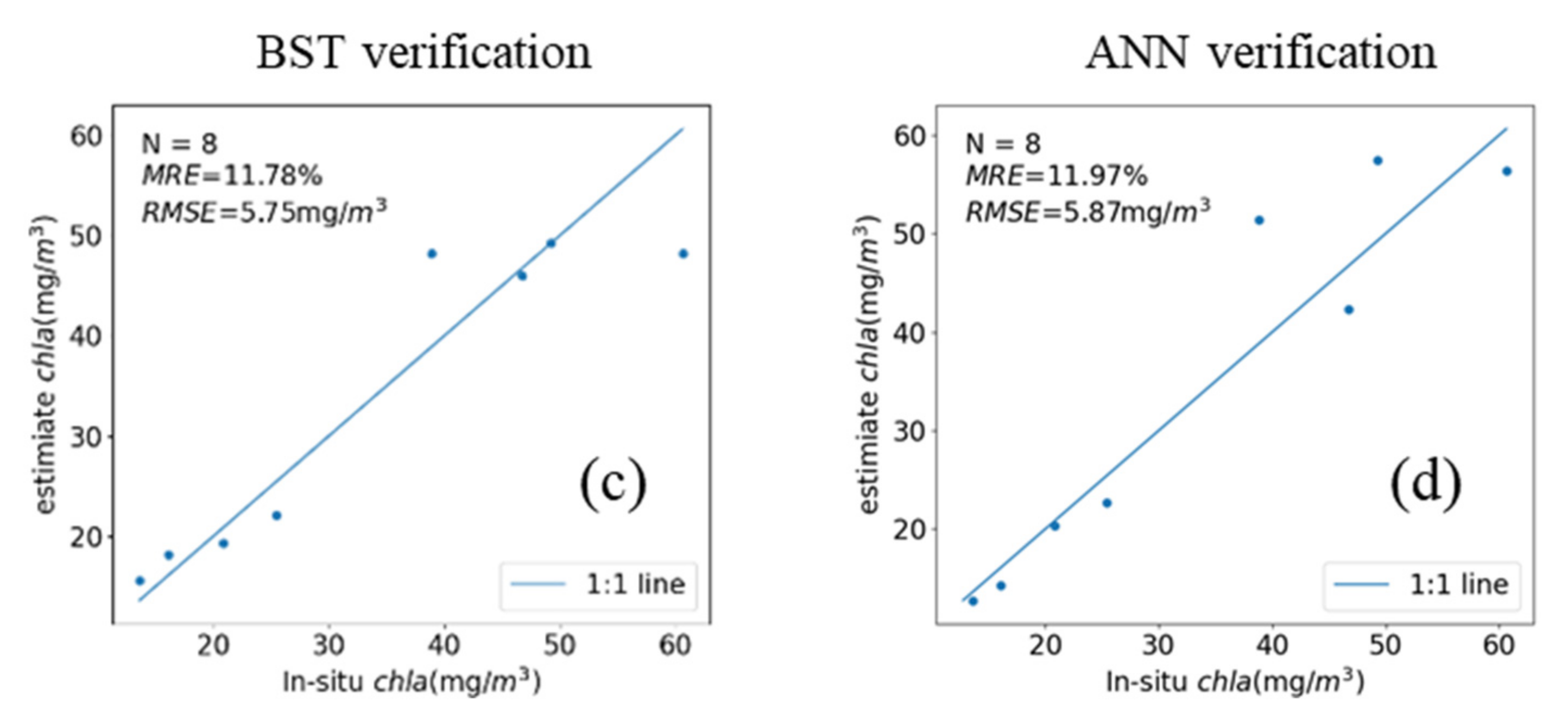
3.2. Machine Learning Model

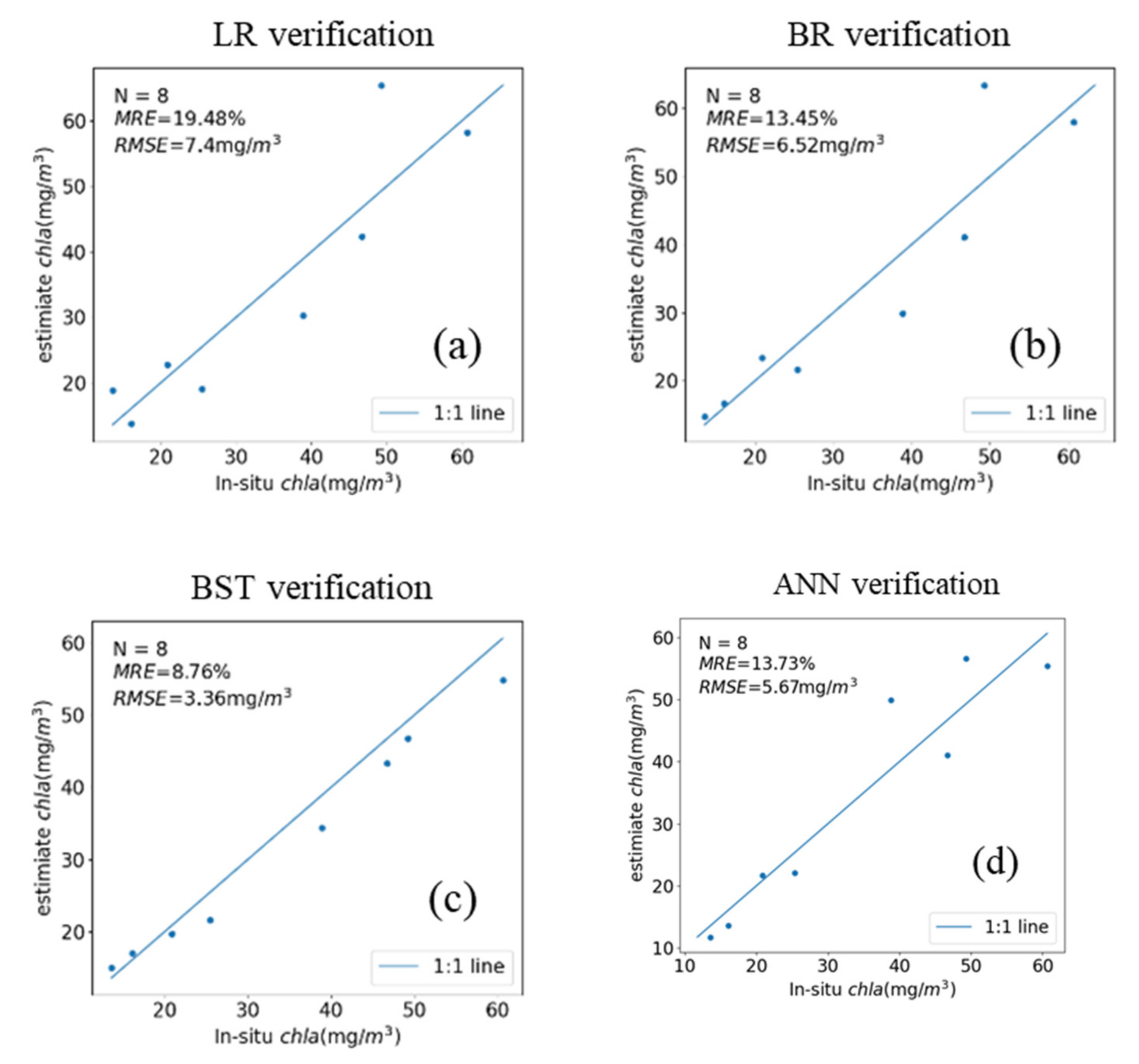
3.2.1. Fused Gaofen-6 Machine Learning Model

For fused Gaofen-6, we used nine inputs for model comparison: First, we determined the hyperparameters of LR, BR, BST, and ANN, using the classic sklearn’s grid search method. The hyperparameters of the LR include defaults, BR includes 0.02 alpha, BST includes 30 trees and eight layer depth, ANN includes 10 × 10 neurones, ReLU activation, and the 1000 s maximum iteration. The four machine learning model accuracy is shown in Appendix A Table A3. Based on the verification diagram (Figure 9), the MRE and RMSE of all models were <20% and 8 mg/m3, respectively; however, the BST and RMSE of the models are 8.76% and 3.36 mg/m3, respectively. Thus, BST was assumed to be the best model.

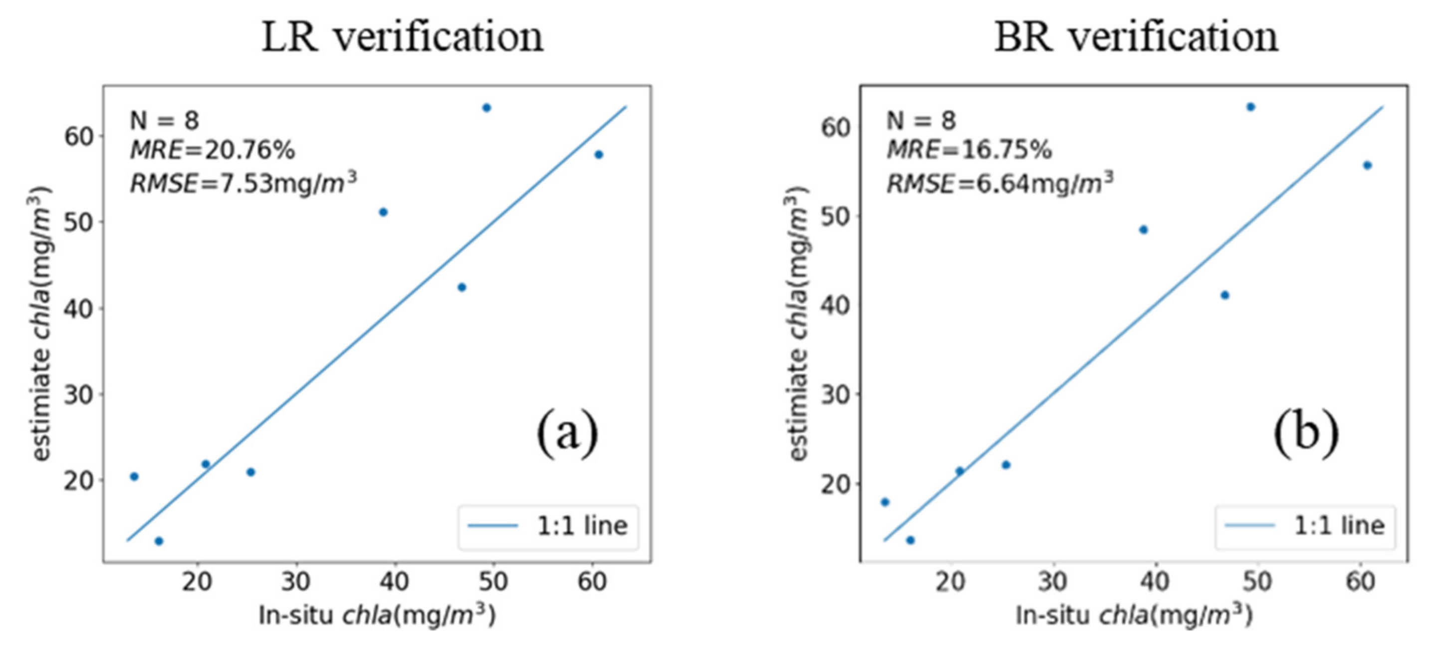
3.2.2. Sentinel-2 Machine Learning Model

For Sentinel-2, we used nine input bands for model comparison: first, we determined the hyperparameters of LR, BR, BST, and ANN, using the classic sklearn grid search method. The hyperparameters of the LR include defaults, BR includes 0.03 alpha, BST includes 10 trees and 15 layer depth, and ANN includes 10 × 10 neurones, ReLU activation, and 1500 maximum iterations. The four machine learning model accuracy is shown in Appendix A Table A4. Based on the verification diagram (Figure 10), the MRE and RMSE of all models were <25% and 8 mg/m3, respectively. However, the BST’s MRE and RMSE were 11.78% and 5.75 mg/m3, respectively. Thus, BST is assumed to be the best model.

3.3. Comparison of Semi-Empirical Model and Machine Learning Model

Since no data was obtained from fused Gaofen-6 in 2016, we discarded the sampling points from the Guanting Reservoir, We used in situ points for the period between 21 August 2019 and 25 October 2019, it was during the summer and autumn seasons, and we confirmed that there was no rainfall for five days around the sampling dates. Water Chla concentrations were more stable during the summer and autumn months. Therefore, we used 38 points from the above-mentioned situation and 20 points from the satellite-ground synoptic for image validation. We used the geometric information of the sampled points to extract the band information of the 58 sampled points on the image, and thereafter, used the quadratic function model and BST models for image estimation verification.
Figure 11 illustrates the quadratic function model reveals a large error in either the fused Gaofen-6 or Sentinel-2 images. The MRE and RMSE were >50% and 28 mg/m3, respectively; it exceeds the maximum allowable error of remotely sensed Chla concentration estimation. However, the BST model exhibited better robustness for both fused Gaofen-6 and Sentinel-2 images. The BST model showed MRE and RMSE values of 6.73% and 3.26 mg/m3 on fused Gaofen-6 images as well as 9.03% and 4.5 mg/m3 on Sentinel-2 images, respectively.
Since the BST model was the best among the fused Gaofen-6 or Sentinel-2, we determined that the BST model is most suitable for estimating Chla concentrations in small water bodies. The BST model is only applicable to the estimation of Chla concentrations in small water bodies during the summer and autumn seasons, as the sampling period for the in situ data is summer and autumn.

4. Discussion

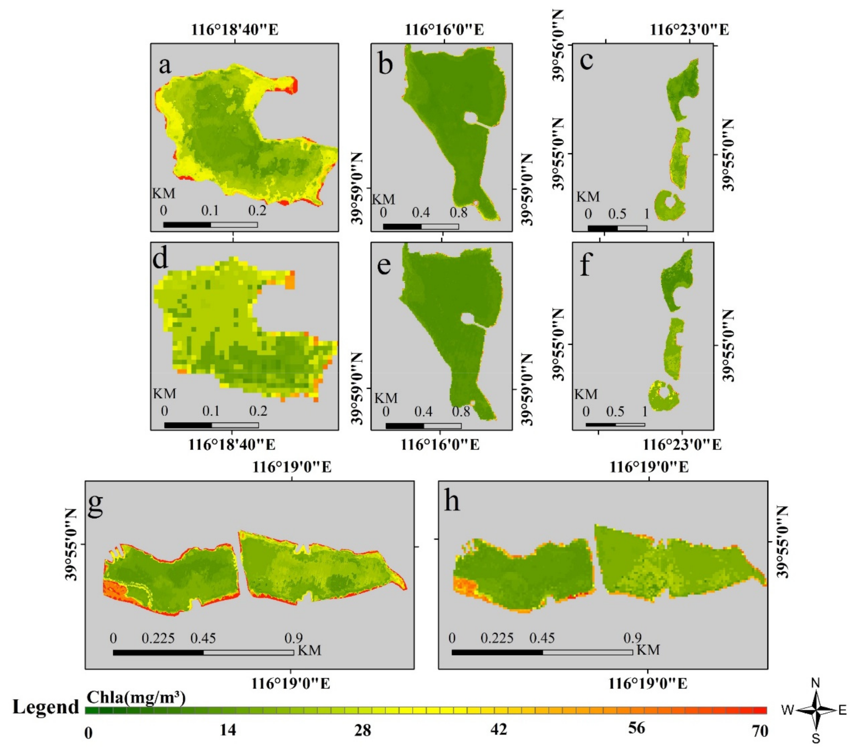
4.1. Comparison of Chla Estimation in Ponds

We compared the results of pond Chla concentrations estimated using the BST model for fused Gaofen-6 and Sentinel-2, they are on the same day, 25 October 2019. Within Figure 12, the subplots a, b, c, and g reveal the results of Chla concentration estimation for fused Gaofen-6, whereas the subplots d, e, f, and h exhibit the results of Chla concentration estimation for Sentinel-2. Considering the Purple Bamboo Park pond, the fused Gaofen-6 estimation results (a) showed higher shore (values 50–60) and low distribution of the lake center (the values between 10–20); however, more meticulous space information was obtained. Moreover, Sentinel-2 monitoring (d) results showed higher shore (values 40–55) and low distribution of the lake center (values 15–25), the low spatial resolution of Sentinel-2 leads to salt and pepper noise in the estimation results. The Summer Palace estimation results showed fused Gaofen-6 (b) exhibiting a trend of being higher on the northwest side (the values between 12–14) and similar in other places (the values between 10–12); the results of Sentinel-2 (e) were similar to those of Gaofen-6 estimation. The Beihai Park estimation results showed that both (c and f) exhibited a spatial distribution with high middle (values 15–22) and low sides (10–15). The Yuyuantan Park estimation results showed that the fused Gaofen-6 estimation results (g) exhibited higher shore (values 30–60) and low distribution of the lake center (values 10–20). the spatial patterns in the results from Gaofen-6 and Sentinel-2 (h) are different. They show advantages of Gaofen-6 with high spatial- resolution. Thus, the fused Gaofen-6 estimation produced more detailed spatial information than Sentinel-2 when monitoring the Chla concentrations in small water bodies. Comparing the results of Chla concentrations from the fused Gaofen-6 and Sentinel-2 estimates, only the Purple Bamboo Park pond estimation was inconsistent. This can be explained by the fact that the Purple Bamboo Park pond area was smaller, and Sentinel-2 Salt and Pepper Noise was serious, which indicated different estimation results between the fused Gaofen-6 and Sentinel-2.

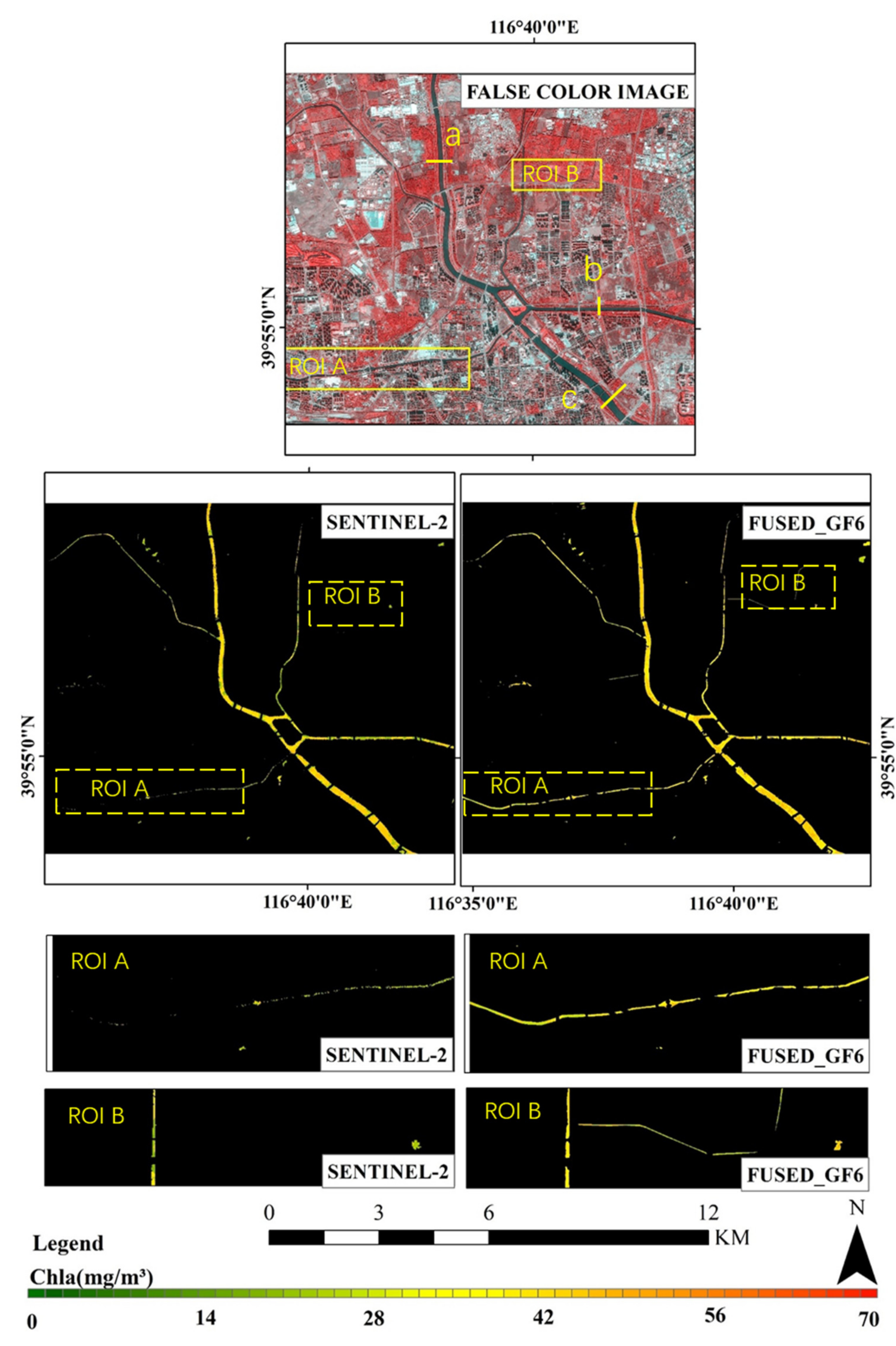
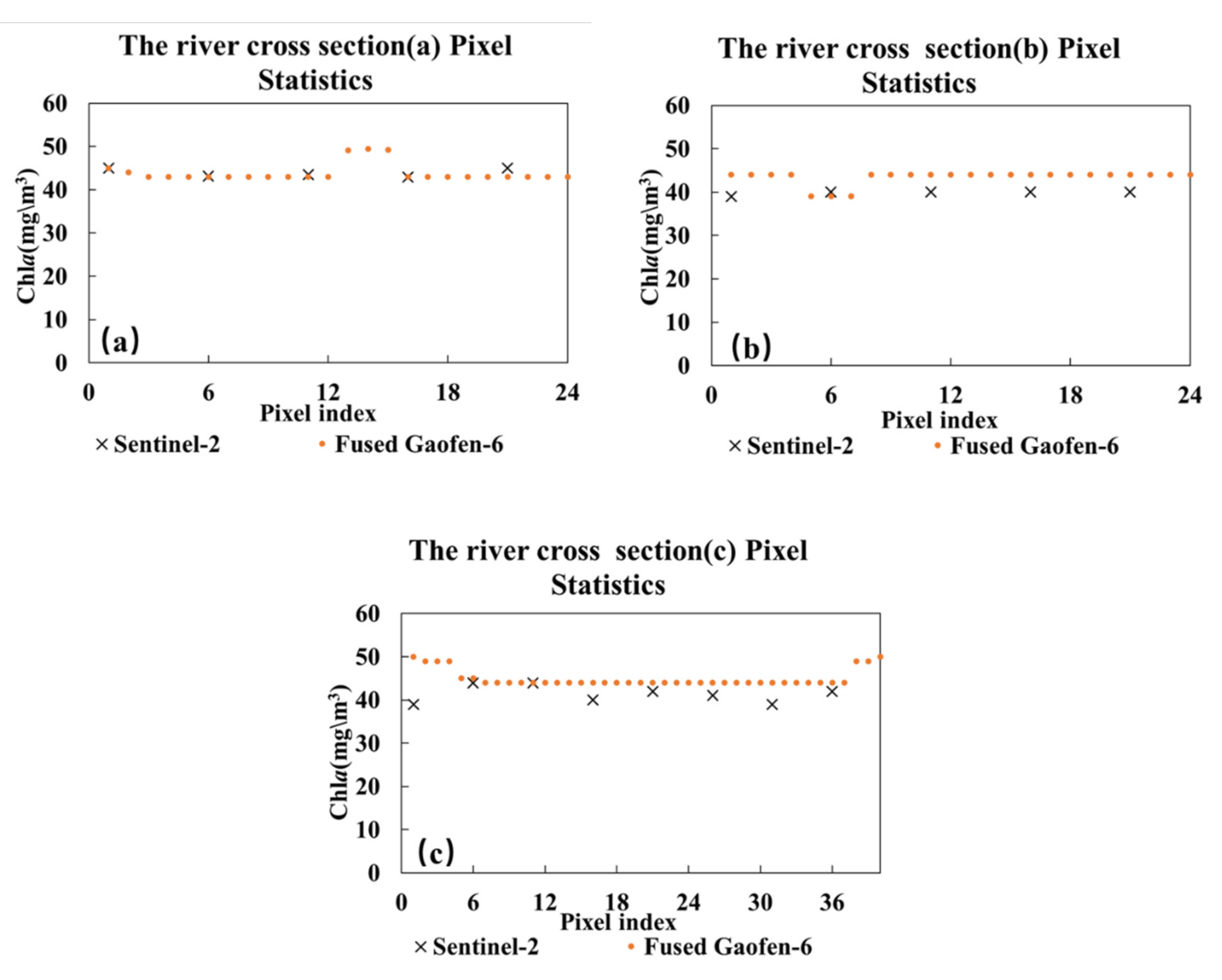
4.2. Comparison of Chla Estimation in the Rivers

In this section, we compared the results of the estimated Chla concentrations in small rivers using the BST model for fused Gaofen-6 and Sentinel-2, they are on the same day, 25 October 2019. The confluence of the Wenyu River and North Canal in Beijing was selected as a case study due to its large watershed and rich river width. While monitoring small water bodies via remote sensing, we selected pure water body image elements of rivers to evaluate Chla and avoid the influence of mixed image elements along the banks; therefore, we only monitored rivers with river widths greater than three pixels; (a) the Wenyu River section (Figure 13a), (b) the Yunchaojian River section (Figure 13b), and (c) the Beiyun River section (Figure 13c). The NDWI [57] was also used, and water bodies with a threshold value > 0.15 were subjected to water body extraction and Chla estimation; the estimation results are depicted in Figure 13. ROI A represents the Tonghui River while ROI B represents the Zhongba River, both of which are less than 10 m wide. Both ROI A and B can be monitored for water body information using the fused Gaofen-6, but no water body information can be obtained using Sentinel-2. Compare Sentinel-2, fused Gaofen-6 exhibit a higher spatial resolution, and can be monitored in narrower rivers.
We used (a), (b), and (c) to estimate the river section drawing and estimation consistency studies (Figure 14). In (a), Sentinel-2 showed values of 42–45, while fused Gaofen-6 produced values between 41–50; in (b), Sentinel-2 showed values of 38–40, while fused Gaofen-6 produced values between 40–45; and in (c), Sentinel-2 showed values of 38–40, while fused Gaofen-6 produced values between 43–52. We used the mean values as true values to calculate the relative errors (TMRE) of different sensors. The values of (a) are 9.7%, 4.8%, and 4.8%; those of (b) are 12.4%, 10%, and 2.4%; and those of (c) are 8%, 8%, and 0.4%. All TMREs were below 15%, and their consistency was still better. The difference between fused Gaofen-6 and Sentinel-2 estimated Chla concentration indicates that it is within the uncertainty of the estimate.

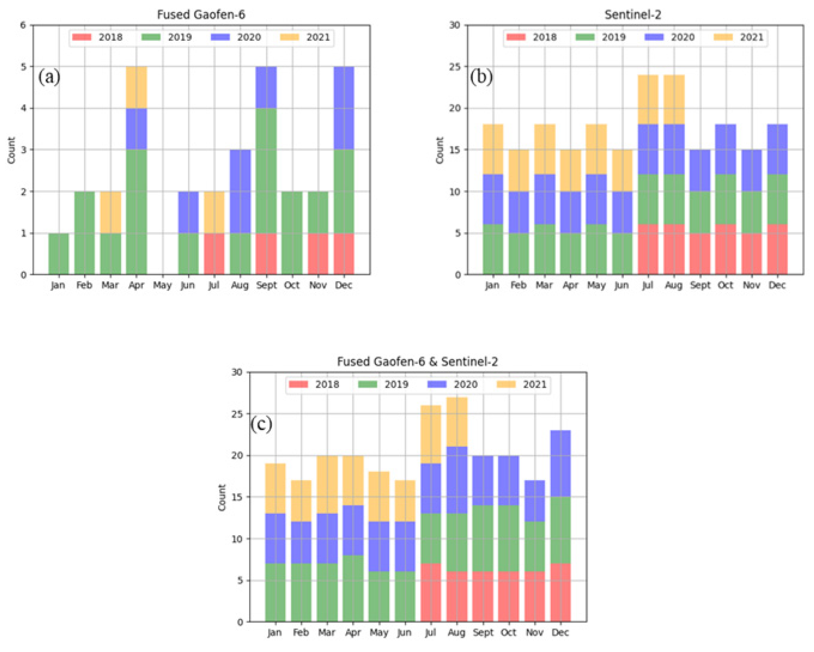
4.3. Fused Gaofen-6 and Sentinel-2 Monitoring Frequency

Water bodies change relatively quickly and higher monitoring frequencies can lead to more accurate monitoring results. The satellite orbit of the Gaofen-6 is not fixed, but the satellite orbit of the Sentinel-2 is fixed. Therefore we need to count the monitoring frequency. Here, we used the fused Gaofen-6 and Sentinel-2 monitoring of water bodies in Beijing as an example.
To examine the temporal resolution, we used data from the fused Gaofen-6 and Sentinel-2 from July 2018 to July 2021 to detect the complete number of images of the built-up area of Beijing. Although the orbit of fused Gaofen-6 is not fixed and the number of images varies each month, it meets the frequency of quarterly observation (Figure 15a). Since Sentinel-2 has a fixed orbit, it guarantees a fixed number of images every month and meets the monthly requirements (Figure 15b), jointly using both sensors can have more images to monitor small water bodies Chla month changes (Figure 15c).
Temporal resolution and spatial resolution are important factors in the ability to monitor small bodies of water by remote sensing of images. Thus, different sensors should be used according to the time scale, river width, and study area scale. The fused Gaofen-6 can provide more detailed information with roughly the same detection range, while the higher frequency river monitoring of Sentinel-2 provides better temporal resolution.

5. Conclusions

In this study, we compared the Chla concentration estimation results for fused Gaofen-6 (with 2 m spatial resolution, eight bands, and 90 km width) and Sentinel-2 (with 10 m spatial resolution, 13 bands, and 100 km width) and obtained the following conclusions.
When comparing the five semi-empirical and four machine learning models, the quadratic model performed best in the semi-empirical model and the BST model performed best in the machine learning model. Both fused Gaofen-6 and Sentinel-2 are the most accurate machine learning models, and the best model is the extreme gradient boosting tree model, which combines Gaofen-6 and Sentinel-2 MRE, with RMSE values of 6.73% and 3.26 mg/m3 as well as 9.03% and 4.5 mg/m3. this study fused the Gaofen-6 PMS and WFV images into 2 m resolution eight-band images, which can be applied to applications other than water body monitoring.
The fused Gaofen-6 and Sentinel-2 have similar abilities to estimate Chla concentration for small water bodies. The fused Gaofen-6 exhibited a higher spatial resolution, it can monitor smaller bodies of water, such as narrower rivers and smaller ponds. While the Sentinel-2 exhibited a higher temporal resolution for monitoring small water bodies.

Author Contributions

Conceptualisation, J.S. and Q.S.; project administration, Y.Y. and J.L.; writing—original draft preparation, J.S.; writing—review and editing, Q.S.; validation, R.W. and W.X.; supervision, F.C. and Z.G.; methodology, L.W. and Y.Z. All authors have read and agreed to the published version of the manuscript.

Funding

This research was funded by National Key Research and Development Program of China under Grants, grant number 2021YFB3901101.

Institutional Review Board Statement

Not applicable.

Informed Consent Statement

Not applicable.

Data Availability Statement

The data presented in this study are available on request from the corresponding author.

Acknowledgments

We are also thankful to all anonymous reviewers for their constructive comments provided on the study.

Conflicts of Interest

The authors declare no conflict of interest.

Appendix A

Table A1. Comparison of this study’s Semi-empirical algorithms with existing algorithms for estimating Chla concentrations in inland water environments. Sentinel-2 MSI; Normalized Difference Chlorophyll Index; three bands algorithm; modified three bands algorithm.
AlgorithmVariable (x)FormulaR2RMSE (mg/m3)MRE
NDCI [58](Rrs (705) − Rrs (665))
/(Rrs (705) + Rrs (665))
Chla = 745.08x2 + 159.37x + 20.3540.877.1311.17
3BDA [59](1/Rrs (665) − 1/Rrs (705)) × Rrs (740)Chla = 743.73x2 + 225.02x + 20.5170.887.8411.89
YA10 [60](Rrs−1 (665) − Rrs−1 (705))
/(Rrs−1 (754) − Rrs−1 (705))
Chla = 262.04x2 + 144.71x + 20.4050.867.6711.79
This studyRrs (705)/Rrs (665)Chla = 126.45x2 − 178.9x + 72.9760.887.7912.21
Table A2. Comparison of this study’s Semi-empirical algorithms with existing algorithms for estimating Chla concentrations in inland water environments. Fused Gaofen-6; Normalized Difference Chlorophyll Index; three bands algorithm; modified three bands algorithm.
AlgorithmVariable (x)FormulaR2RMSE (mg/m3)MRE
NDCI [58](Rrs (705) − Rrs (665))
/(Rrs (705) + Rrs (665))
Chla = 1051.1x2 + 323.98x + 38.2290.746.3013.11
3BDA [59](1/Rrs (665) − 1/Rrs (705)) × Rrs (740)Chla = 2040.4x2 + 474.61x + 37.7720.787.2811.39
YA10 [60](Rrs−1 (665) − Rrs−1 (705))
/(Rrs−1 (754) − Rrs−1 (705))
Chla = 864.57x2 + 307.18x + 37.220.787.9613.62
This studyRrs (705)/Rrs (665)Chla = 304.42x2 − 435.6x + 169.140.786.8813.64
Table A3. Machine learning estimation models of Chla concentration in fused Gaofen-6 on training set and validation sets: R2, MRE, and RMSE.
AlgorithmR2RMSE (mg/m3)MRE
LR0.924.7219.33
BR0.924.7219.33
BST0.914.5512.56
ANN0.923.3816.67
Table A4. Machine learning estimation models of Chla concentration in Sentinel-2 on training set and validation sets: R2, MRE, and RMSE.
AlgorithmR2RMSE (mg/m3)MRE
LR0.962.3111.56
BR0.953.8311.14
BST0.953.3210.90
ANN0.963.0510.82

References

  1. Palmer, S.C.J.; Kutser, T.; Hunter, P.D. Remote sensing of inland waters: Challenges, progress and future directions. Remote Sens. Environ. 2015, 157, 1–8. [Google Scholar] [CrossRef] [Green Version]
  2. Conkright, M.E.; Gregg, W.W. Comparison of global chlorophyll climatologies: In situ, CZCS, Blended in situ-CZCS and SeaWiFS. Int. J. Remote Sens. 2003, 24, 969–991. [Google Scholar] [CrossRef]
  3. Gholizadeh, M.H.; Melesse, A.M.; Reddi, L. A comprehensive review on water quality parameters estimation using remote sensing techniques. Sensors 2016, 16, 1298. [Google Scholar] [CrossRef] [Green Version]
  4. Moses, W.J.; Gitelson, A.A.; Berdnikov, S.; Saprygin, V.; Povazhnyi, V. Operational MERIS-based NIR-red algorithms for estimating chlorophyll-a concentrations in coastal waters—The Azov Sea case study. Remote Sens. Environ. 2012, 121, 118–124. [Google Scholar] [CrossRef] [Green Version]
  5. Augusto-Silva, P.B.; Ogashawara, I.; Barbosa, C.C.F.; De Carvalho, L.A.S.; Jorge, D.S.F.; Fornari, C.I.; Stech, J.L. Analysis of MERIS reflectance algorithms for estimating chlorophyll-a concentration in a Brazilian reservoir. Remote Sens. 2014, 6, 11689–11707. [Google Scholar] [CrossRef] [Green Version]
  6. Ogashawara, I.; Alcântara, E.; Curtarelli, M.; Adami, M.; Nascimento, R.; Souza, A.; Stech, J.; Kampel, M. Performance analysis of MODIS 500-m spatial resolution products for estimating chlorophyll-a concentrations in oligo- to meso-trophic waters case study: Itumbiara Reservoir, Brazil. Remote Sens. 2014, 6, 1634–1653. [Google Scholar] [CrossRef] [Green Version]
  7. Li, J.; Gao, M.; Feng, L.; Zhao, H.; Shen, Q.; Zhang, F.; Wang, S.; Zhang, B. Estimation of chlorophyll-a concentrations in a highly turbid eutrophic lake using a classification-based MODIS land-band algorithm. IEEE J. Sel. Top. Appl. Earth Obs. Remote Sens. 2019, 12, 3769–3783. [Google Scholar] [CrossRef]
  8. Li, J.; Yin, Z.; Lu, Z.; Ye, Y.; Zhang, F.; Shen, Q.; Zhang, B. Regional vicarious calibration of the SWIR-based atmospheric correction approach for MODIS-Aqua measurements of highly turbid inland water. Remote Sens. 2019, 11, 1670. [Google Scholar] [CrossRef] [Green Version]
  9. Wang, M.H.; Son, S. VIIRS-derived chlorophyll-a using the ocean color index method. Remote Sens. Environ. 2016, 182, 141–149. [Google Scholar] [CrossRef]
  10. Kim, W.; Moon, J.E.; Park, Y.J.; Ishizaka, J. Evaluation of chlorophyll retrievals from Geostationary Ocean Color Imager (GOCI) for the North-East Asian Region. Remote Sens. Environ. 2016, 184, 482–495. [Google Scholar] [CrossRef]
  11. Werther, M.; Spyrakos, E.; Simis, S.G.H.; Odermatt, D.; Stelzer, K.; Krawczyk, H.; Berlage, O.; Hunter, P.; Tyler, A. Meta-classification of remote sensing reflectance to estimate trophic status of inland and nearshore waters. ISPRS J. Photogramm. Remote Sens. 2021, 176, 109–126. [Google Scholar] [CrossRef]
  12. Kravitz, J.; Matthews, M.; Bernard, S.; Griffith, D. Application of Sentinel 3 OLCI for chl-a retrieval over small inland water targets: Successes and challenges. Remote Sens. Environ. 2020, 237, 111562. [Google Scholar] [CrossRef]
  13. Hori, M. Near-daily monitoring of surface temperature and channel width of the six largest Arctic rivers from space using GCOM-C/SGLI. Remote Sens. Environ. 2021, 263, 112538. [Google Scholar] [CrossRef]
  14. Xu, Y.; He, X.; Bai, Y.; Wang, D.; Zhu, Q.; Ding, X. Evaluation of Remote-Sensing Reflectance Products from Multiple Ocean Color Missions in Highly Turbid Water (Hangzhou Bay). Remote Sens. 2021, 13, 4267. [Google Scholar] [CrossRef]
  15. Hori, M.; Murakami, H.; Miyazaki, R.; Honda, Y.; Nasahara, K.; Kajiwara, K.; Nakajima, T.Y.; Irie, H.; Toratani, M.; Hirawake, T.; et al. GCOM-C Data Validation Plan for Land, Atmosphere, Ocean, and Cryosphere. Trans. Jpn. Soc. Aeronaut. Spaceences Aerosp. Technol. Jpn. 2018, 16, 218–223. [Google Scholar] [CrossRef] [Green Version]
  16. Ilori, C.; Pahlevan, N.; Knudby, A. Analyzing performances of different atmospheric correction techniques for Landsat 8: Application for coastal remote sensing. Remote Sens. 2019, 11, 469. [Google Scholar] [CrossRef] [Green Version]
  17. Kuhn, C.; de Matos Valerio, A.; Ward, N.; Loken, L.; Sawakuchi, H.O.; Kampel, M.; Richey, J.; Stadler, P.; Crawford, J.; Striegl, R.; et al. Performance of Landsat-8 and Sentinel-2 surface reflectance products for river remote sensing retrievals of chlorophyll-a and turbidity. Remote Sens. Environ. 2019, 224, 104–118. [Google Scholar] [CrossRef] [Green Version]
  18. Pu, F.; Ding, C.; Chao, Z.; Yu, Y.; Xu, X. Water-quality classification of inland lakes using Landsat8 images by convolutional neural networks. Remote Sens. 2019, 11, 1674. [Google Scholar] [CrossRef] [Green Version]
  19. Cao, Z.; Ma, R.; Duan, H.; Pahlevan, N.; Melack, J.; Shen, M.; Xue, K. A machine learning approach to estimate chlorophyll-a from Landsat-8 measurements in inland lakes. Remote Sens. Environ. 2020, 248, 111974. [Google Scholar] [CrossRef]
  20. Markogianni, V.; Kalivas, D.; Petropoulos, G.P.; Dimitriou, E. Estimating chlorophyll-a of inland water bodies in Greece based on Landsat data. Remote Sens. 2020, 12, 2087. [Google Scholar] [CrossRef]
  21. Ogashawara, I.; Jechow, A.; Kiel, C.; Kohnert, K.; Berger, S.A.; Wollrab, S. Performance of the Landsat 8 provisional aquatic reflectance product for inland waters. Remote Sens. 2020, 12, 2410. [Google Scholar] [CrossRef]
  22. Somasundaram, D.; Zhang, F.; Ediriweera, S.; Wang, S.; Yin, Z.; Li, J.; Zhang, B. Patterns, trends and drivers of water transparency in Sri Lanka using Landsat 8 observations and Google Earth Engine. Remote Sens. 2021, 13, 2193. [Google Scholar] [CrossRef]
  23. Asim, M.; Brekke, C.; Mahmood, A.; Eltoft, T.; Reigstad, M. Improving chlorophyll-a estimation from Sentinel-2 (MSI) in the Barents Sea using machine learning. IEEE J. Sel. Top. Appl. Earth Obs. Remote Sens. 2021, 14, 5529–5549. [Google Scholar] [CrossRef]
  24. Niroumand-Jadidi, M.; Bovolo, F.; Bruzzone, L.; Gege, P. Inter-comparison of methods for chlorophyll-a retrieval: Sentinel-2 time-series analysis in Italian lakes. Remote Sens. 2021, 13, 2381. [Google Scholar] [CrossRef]
  25. Ogashawara, I.; Kiel, C.; Jechow, A.; Kohnert, K.; Ruhtz, T.; Grossart, H.-P.; Hölker, F.; Nejstgaard, J.C.; Berger, S.A.; Wollrab, S. The use of Sentinel-2 for chlorophyll-a spatial dynamics assessment: A comparative study on different lakes in northern Germany. Remote Sens. 2021, 13, 1542. [Google Scholar] [CrossRef]
  26. Perrone, M.; Scalici, M.; Conti, L.; Moravec, D.; Kropáček, J.; Sighicelli, M.; Lecce, F.; Malavasi, M. Water mixing conditions influence Sentinel-2 monitoring of chlorophyll content in monomictic lakes. Remote Sens. 2021, 13, 2699. [Google Scholar] [CrossRef]
  27. Sent, G.; Biguino, B.; Favareto, L.; Cruz, J.; Sá, C.; Dogliotti, A.I.; Palma, C.; Brotas, V.; Brito, A.C. Deriving water quality parameters using Sentinel-2 imagery: A case study in the Sado Estuary, Portugal. Remote Sens. 2021, 13, 1043. [Google Scholar] [CrossRef]
  28. Zhai, Z.K.; Lu, S.L.; Wang, P.; Wang, C.; Tang, H.L.; Liu, D.Y.; Han, Q.Y.; Guo, J.; Liu, X.H.; Wei, T.L. Ocean chlorophyll-a retrieval using GF1-WFV data-a case study of the central Bohai Sea. In Proceedings of the 2nd International Conference on Advances in Civil and Ecological Engineering Research (ACEER), Beijing, China, 20–23 October 2020. [Google Scholar]
  29. Cao, Y.; Ye, Y.; Zhao, H.; Jiang, Y.; Wang, H.; Shang, Y.; Wang, J. Remote sensing of water quality based on HJ-1A HSI imagery with modified discrete binary particle swarm optimization-partial least squares (MDBPSO-PLS) in inland waters: A case in Weishan Lake. Ecol. Inform. 2018, 44, 21–32. [Google Scholar] [CrossRef]
  30. Wang, X.; Gong, Z.; Pu, R. Estimation of chlorophyll a content in inland turbidity waters using WorldView-2 imagery: A case study of the Guanting Reservoir, Beijing, China. Environ. Monit. Assess. 2018, 190, 620. [Google Scholar] [CrossRef]
  31. Zhao, L.; Qi, J.; Ren, Z.; Zhu, J. Shallow water bathymetry retrieving of optical remote sensing combined with SVM bottom classification. In Proceedings of the 2020 IEEE 5th International Conference on Signal and Image Processing (ICSIP), Nanjing, China, 3–5 July 2020; pp. 530–534. [Google Scholar]
  32. Rotta, L.H.; Alcântara, E.H.; Watanabe, F.S.; Rodrigues, T.W.; Imai, N.N. Atmospheric correction assessment of SPOT-6 image and its influence on models to estimate water column transparency in tropical reservoir. Remote Sens. Appl. Soc. Environ. 2016, 4, 158–166. [Google Scholar] [CrossRef]
  33. Mansaray, A.S.; Dzialowski, A.R.; Martin, M.E.; Wagner, K.L.; Gholizadeh, H.; Stoodley, S.H. Comparing PlanetScope to Landsat-8 and Sentinel-2 for Sensing Water Quality in Reservoirs in Agricultural Watersheds. Remote Sens. 2021, 13, 1847. [Google Scholar] [CrossRef]
  34. Matthews, M.W. A current review of empirical procedures of remote sensing in inland and near-coastal transitional waters. Int. J. Remote Sens. 2011, 32, 6855–6899. [Google Scholar] [CrossRef]
  35. Konik, M.; Kowalczuk, P.; Zabłocka, M.; Makarewicz, A.; Meler, J.; Zdun, A.; Darecki, M. Empirical relationships between remote-sensing reflectance and selected inherent optical properties in Nordic Sea surface waters for the MODIS and OLCI ocean colour sensors. Remote Sens. 2020, 12, 2774. [Google Scholar] [CrossRef]
  36. Zhang, R.; Zheng, Z.; Liu, G.; Du, C.; Du, C.; Lei, S.; Xu, Y.; Xu, J.; Mu, M.; Bi, S.; et al. Simulation and assessment of the capabilities of Orbita Hyperspectral (OHS) imagery for remotely monitoring chlorophyll-a in eutrophic plateau lakes. Remote Sens. 2021, 13, 2821. [Google Scholar] [CrossRef]
  37. Gitelson, A.; Dall’Olmo, G.; Moses, W.; Rundquist, D.C.; Serenko, V. A semi-analytical model for remote estimation of chlorophyll-a in turbid productive waters: Calibration and Validation. Int. J. Adv. Comput. Res. 2008, 2008, GC41A-0696. [Google Scholar]
  38. Jorge, D.S.F.; Loisel, H.; Jamet, C.; Dessailly, D.; Demaria, J.; Bricaud, A.; Maritorena, S.; Zhang, X.; Antoine, D.; Kutser, T.; et al. A three-step semi analytical algorithm (3SAA) for estimating inherent optical properties over oceanic, coastal, and inland waters from remote sensing reflectance. Remote Sens. Environ. 2021, 263, 112537. [Google Scholar] [CrossRef]
  39. Dall’Olmo, G.; Gitelson, A.A. Effect of bio-optical parameter variability on the remote estimation of chlorophyll-a concentration in turbid productive waters: Experimental results. Appl. Opt. 2005, 44, 411–422. [Google Scholar]
  40. Botha, E.J.; Anstee, J.M.; Sagar, S.; Lehmann, E.; Medeiros, T.A.G. Classification of Australian waterbodies across a wide range of optical water types. Remote Sens. 2020, 12, 3018. [Google Scholar] [CrossRef]
  41. Zhang, F.; Li, J.; Shen, Q.; Zhang, B.; Tian, L.; Ye, H.; Wang, S.; Lu, Z. A soft-classification-based chlorophyll-a estimation method using MERIS data in the highly turbid and eutrophic Taihu Lake. Int. J. Appl. Earth Obs. Geoinf. 2019, 74, 138–149. [Google Scholar] [CrossRef]
  42. Zhu, S.; Mao, J. A machine learning approach for estimating the trophic state of urban waters based on remote sensing and environmental factors. Remote Sens. 2021, 13, 2498. [Google Scholar] [CrossRef]
  43. Xie, F.; Tao, Z.; Zhou, X.; Lv, T.; Wang, J.; Li, R. A prediction model of water in situ data change under the influence of environmental variables in remote sensing validation. Remote Sens. 2020, 13, 70. [Google Scholar] [CrossRef]
  44. Watanabe, F.S.Y.; Miyoshi, G.T.; Rodrigues, T.W.P.; Bernardo, N.M.R.; Rotta, L.H.S.; Alcântara, E.; Imai, N.N. Inland water’s trophic status classification based on machine learning and remote sensing data. Remote Sens. Appl. Soc. Environ. 2020, 19, 100326. [Google Scholar] [CrossRef]
  45. Sun, X.; Zhang, Y.; Zhang, Y.; Shi, K.; Zhou, Y.; Li, N. Machine learning algorithms for chromophoric dissolved organic matter (CDOM) estimation based on Landsat 8 images. Remote Sens. 2021, 13, 3560. [Google Scholar] [CrossRef]
  46. Su, H.; Lu, X.; Chen, Z.; Zhang, H.; Lu, W.; Wu, W. Estimating coastal chlorophyll-a concentration from time-series OLCI data based on machine learning. Remote Sens. 2021, 13, 576. [Google Scholar] [CrossRef]
  47. Li, T.; Zhu, B.; Cao, F.; Sun, H.; He, X.; Liu, M.; Gong, F.; Bai, Y. Monitoring changes in the transparency of the largest reservoir in eastern China in the past decade, 2013–2020. Remote Sens. 2021, 13, 2570. [Google Scholar] [CrossRef]
  48. Hafeez, S.; Wong, M.; Ho, H.; Nazeer, M.; Nichol, J.; Abbas, S.; Tang, D.; Lee, K.; Pun, L. Comparison of machine learning algorithms for retrieval of water quality indicators in case-II waters: A case study of Hong Kong. Remote Sens. 2019, 11, 617. [Google Scholar] [CrossRef] [Green Version]
  49. Awad, M. Sea water chlorophyll-a estimation using hyperspectral images and supervised artificial neural network. Ecol. Inform. 2014, 24, 60–68. [Google Scholar] [CrossRef]
  50. Mobley, C.D. Estimation of the remote-sensing reflectance from above-surface measurements. Appl. Opt. 1999, 38, 7442–7455. [Google Scholar] [CrossRef]
  51. Tang, J.; Guo, T.; Wang, X.; Wang, X.; Song, Q.J.J.o.R.S. The methods of water spectra measurement and analysis I: Above-water method. J. Remote Sens. 2004, 8, 37–44. [Google Scholar]
  52. Shi, K.; Zhang, Y.; Zhou, Y.; Liu, X.; Zhu, G.; Qin, B.; Gao, G.J.R. Long-term MODIS observations of cyanobacterial dynamics in Lake Taihu: Responses to nutrient enrichment and meteorological factors. Sci. Rep. 2017, 7, 40326. [Google Scholar] [CrossRef] [Green Version]
  53. Chen, F. Pixel-Pixel Knife High Partial Satellite Processing Software. Available online: https://www.zybuluo.com/novachen/note/426294 (accessed on 16 May 2021).
  54. Long, T.; Jiao, W.; He, G.; Zhang, Z. A Fast and reliable matching method for automated georeferencing of remotely sensed imagery. Remote Sens. 2016, 8, 56. [Google Scholar] [CrossRef] [Green Version]
  55. Canty, M.J.; Nielsen, A.A. Automatic radiometric normalization of multitemporal satellite imagery with the iteratively re-weighted MAD transformation. Remote Sens. Environ. 2008, 112, 1025–1036. [Google Scholar] [CrossRef] [Green Version]
  56. Lanaras, C.; Bioucas-Dias, J.; Galliani, S.; Baltsavias, E.; Schindler, K. Super-resolution of Sentinel-2 images: Learning a globally applicable deep neural network. ISPRS J. Photogramm. 2018, 146, 305–319. [Google Scholar] [CrossRef] [Green Version]
  57. Gao, B. NDWI-A normalized difference water index for remote sensing of vegetation liquid water from space. Remote Sens. Environ. 1996, 58, 257–266. [Google Scholar] [CrossRef]
  58. Mishra, S.; Mishra, D.R. Normalized difference chlorophyll index: A novel model for remote estimation of chlorophyll-a concentration in turbid productive waters. Remote Sens. Environ. 2012, 117, 394–406. [Google Scholar] [CrossRef]
  59. Gurlin, D.; Gitelson, A.A.; Moses, W.J. Remote estimation of chl-a concentration in turbid productive waters—return to a simple two-band NIR-red model? Remote Sens. Environ. 2011, 115, 3479–3490. [Google Scholar] [CrossRef]
  60. Yang, W.; Matsushita, B.; Chen, J.; Fukushima, B.; Ma, R. An enhanced three-band index for estimating chlorophyll-a in turbid case-II waters: Case studies of Lake Kasumigaura, Japan, and Lake Dianchi, China. IEEE Geosci. Remote Sens. Lett. 2010, 7, 655–659. [Google Scholar] [CrossRef] [Green Version]
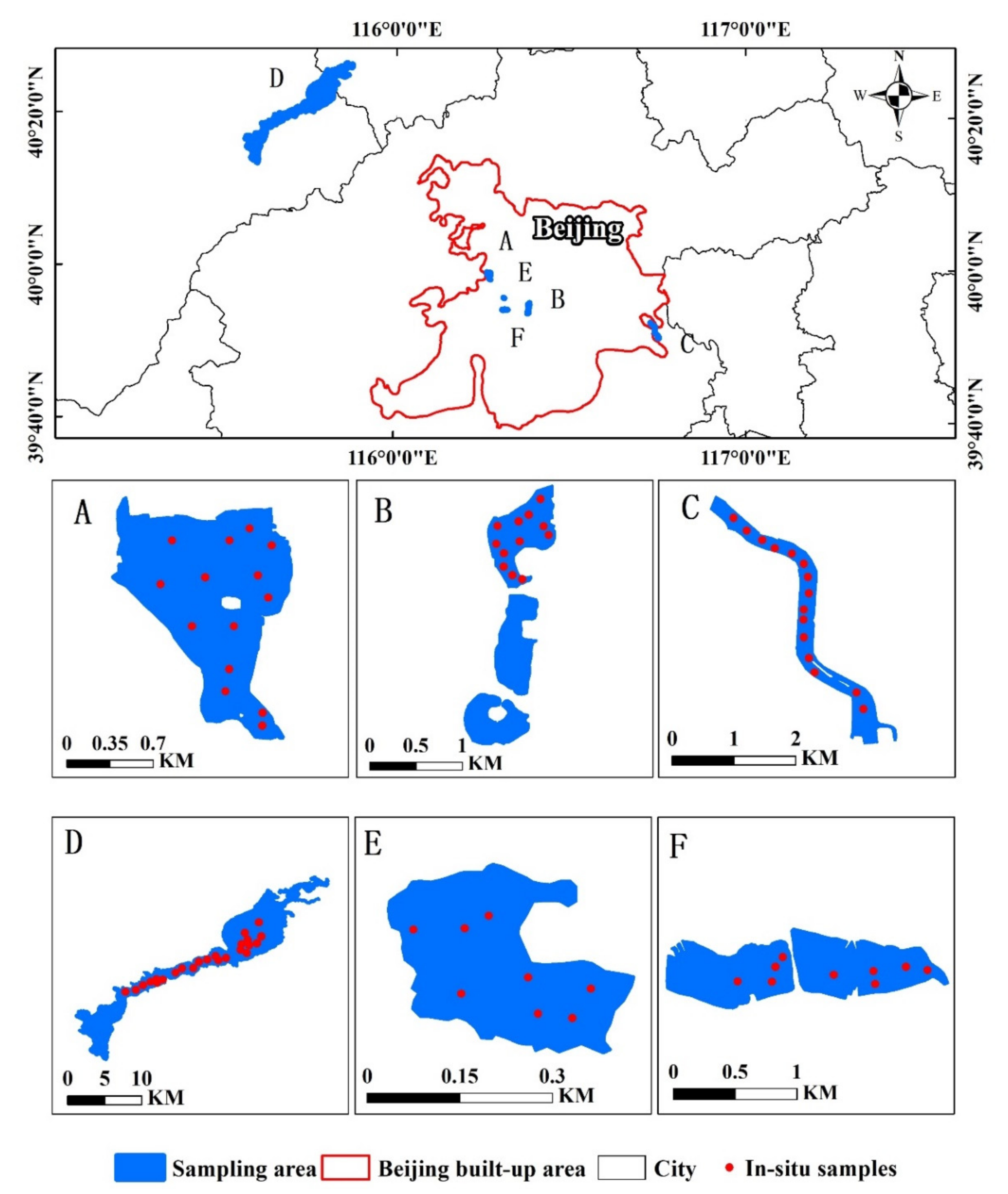
Figure 1. Technology roadmap.
Remotesensing 14 00229 g001
Figure 2. Study area and in situ samples distribution. (A) Summer Palace pond; (B) Beihai Park pond; (C) Grand Canal; (D) Guanting Reservoir; (E) Purple Bamboo Park pond; (F) Yuyuantan Park pond.
Remotesensing 14 00229 g002
Figure 3. Spectral display chart. (a) Spectra based on the study area mean. (b) Fused Gaofen-6 spectral simulation based on in situ spectra. (c) Sentinel-2 spectral simulation based on in situ spectra.
Remotesensing 14 00229 g003
Figure 4. Image pre-processing flow chart.
Remotesensing 14 00229 g004
Figure 5. Band simulation and the atmospheric correction effects. (a) Fused Gaofen-6 and Sentinel-2 band simulation at 400–890 nm. (b) Fused Gaofen-6 atmospheric correction uncertainty evaluation.
Remotesensing 14 00229 g005
Figure 6. Machine learning input feature number selection accuracy chart. input six variables, seven variables, eight variables and nine variables accuracy chart.
Remotesensing 14 00229 g006
Figure 7. Verification of fused Gaofen-6 semi-empirical models. (a) Linear model; (b) exponential model; (c) logarithmic model; (d) power function model; (e) quadratic function model.
Remotesensing 14 00229 g007
Figure 8. Verification of Sentinel-2 semi-empirical models. (a) Linear model; (b) exponential model; (c) logarithmic model; (d) power function model; (e) quadratic function model.
Remotesensing 14 00229 g008
Figure 9. Verification of fused Gaofen-6 machine learning models. (a) LR; (b) BR; (c) BST; (d) ANN.
Remotesensing 14 00229 g009
Figure 10. Verification of Sentinel-2 machine learning models. (a) LR; (b) BR; (c) BST; (d) ANN.
Remotesensing 14 00229 g010aRemotesensing 14 00229 g010b
Figure 11. The verification of four models based on images. (a) Quadratic function model by fused Gaofen-6. (b) Quadratic function model by Sentinel-2. (c) BST model by fused Gaofen-6. (d) BST model by Sentinel-2.
Remotesensing 14 00229 g011
Figure 12. Comparison of fused Gaofen-6 and Sentinel-2 estimation results in the ponds. (a) Fused Gaofen-6 estimation results in the Purple Bamboo Park. (b) Fused Gaofen-6 estimation results in the Summer Palace. (c) Fused Gaofen-6 estimation results in Beihai Park. (d) Sentinel-2 estimation results in the Purple Bamboo Park. (e) Sentinel-2 estimation results in the Summer Palace. (f) Sentinel-2 estimation results in the Beihai Park. (g) Fused Gaofen-6 estimation results in Yuyuantan Park. (h) Sentinel-2 estimation results in the Yuyuantan Park.
Remotesensing 14 00229 g012
Figure 13. Plotted results of the assessment of Chla concentrations using the Sentinel-2 and fused Gaofen-6. (a) the Wenyu River section, (b) the Yunchaojian River section, and (c) the Beiyun River section.
Remotesensing 14 00229 g013
Figure 14. Estimated result in river sectional drawing. (a) Wenyu River sectional drawing; (b) Yunchaojian River sectional drawing. (c) Beiyun River sectional drawing.
Remotesensing 14 00229 g014
Figure 15. Temporal coverage of Fused Gaofen-6 and Sentinel-2 archive from July 2018 to August 2021 used in the Beijing city. (a) Temporal coverage of Fused Gaofen-6. (b) Temporal coverage of Sentinel-2. (c) Temporal coverage of Fused Gaofen-6 and Sentinel-2.
Remotesensing 14 00229 g015
Table 1. In situ dates information table including locations and the numbers of in situ water samples as well as reflectance measurements.
Field Experiment DataIn Situ LocationIn Situ NumbersSymbols in Figure 2
8 September 2016Guanting Reservoir24d
21 August 2019Yuyuantan Park9f
16 September 2019Summer Palace14a
18 September 2019Beihai Park12b
15 October 2019Grand Canal15c
25 October 2019Purple Bamboo Park8e
Table 2. Image information table including sensor, data, image ID, and spatial resolution.
SensorDataIDSpatial Resolution (m)
Gaofen-6 PMS18 September 201911199259352
Gaofen-6 PMS18 September 201911199259442
Gaofen-6 WFV18 September 2019111992631716
Gaofen-6 PMS25 October 201911199382252
Gaofen-6 PMS25 October 201911199382632
Gaofen-6 WFV 25 October 2019111993834716
Sentinel-225 October 2019-10
Table 3. Gaofen-6 and Sentinel-2 similar band setting comparison including band name, band index, band wavelength, and resolution.
Fused Gaofen-6Sentinel-2 MSI
Bands NameBand
Index
Wavelength
(nm)
Resolution
(m)
Band
Index
Wavelength
(nm)
Resolution
(m)
BlueB1450–5202B2458–52310
GreenB2520–5902B3543–57810
RedB3630–6902B4650–68010
NIR B4770–8902B8785–90010
Red-Edge IB5690–7302B5698–71320
Red-Edge II B6730–7702B6733–74820
Coastal aerosolB7400–4502B1433–45360
YellowB8590–6302None
Table 4. Semi-empirical model.
Model FormFormula
Linear modelChla = a × x +b
Exponential modelChla = a × exp (b × x) + c
Logarithmic modelChla = a × power (x, b) + c
Power function model Chla = a × log(x) + b
Quadratic function modelChla = a × x2 + b × x + c
Table 5. Five semi-empirical model formulas for fused Gaofen-6.
Model FormFormula
Linear modelChla = −65.788453 × x + 99.5654
Exponential modelChla = 1485.8 × exp(−3.65197 × x)
Logarithmic modelChla = 37.9778 × power (x, 4.0432)
Power function modelChla = −83.5964 × log(x) + 35.9646
Quadratic function modelChla = 186.537 × x2 − 511.3751 × x + 362.781
Table 6. Sentinel-2 Semi-empirical model formulas.
Model FormFormula
Linear modelChla = −83.028 × x + 107.0218
Exponential modelChla = 1139.618 × exp (−3.98529 × x)
Logarithmic modelChla = 20.76 × power (x, 3.6926)
Power function model Chla = −85.2146 × log(x) + 23.37083
Quadratic function modelChla = 119.624 × x2 − 485.476 × x + 306.563
Publisher’s Note: MDPI stays neutral with regard to jurisdictional claims in published maps and institutional affiliations.

