
Hyperspectral Image Classification Based on 3D Coordination Attention Mechanism Network


1
College of Communication and Electronic Engineering, Qiqihar University, Qiqihar 161000, China
2
College of Information and Communication Engineering, Dalian Nationalities University, Dalian 116000, China
*
Author to whom correspondence should be addressed.
Remote Sens. 2022, 14(3), 608; https://0-doi-org.brum.beds.ac.uk/10.3390/rs14030608
Submission received: 26 December 2021
/
Revised: 11 January 2022
/
Accepted: 19 January 2022
/
Published: 27 January 2022
(This article belongs to the Special Issue Deep Reinforcement Learning in Remote Sensing Image Processing)
Abstract
:In recent years, due to its powerful feature extraction ability, the deep learning method has been widely used in hyperspectral image classification tasks. However, the features extracted by classical deep learning methods have limited discrimination ability, resulting in unsatisfactory classification performance. In addition, due to the limited data samples of hyperspectral images (HSIs), how to achieve high classification performance under limited samples is also a research hotspot. In order to solve the above problems, this paper proposes a deep learning network framework named the three-dimensional coordination attention mechanism network (3DCAMNet). In this paper, a three-dimensional coordination attention mechanism (3DCAM) is designed. This attention mechanism can not only obtain the long-distance dependence of the spatial position of HSIs in the vertical and horizontal directions, but also obtain the difference of importance between different spectral bands. In order to extract the spectral and spatial information of HSIs more fully, a convolution module based on convolutional neural network (CNN) is adopted in this paper. In addition, the linear module is introduced after the convolution module, which can extract more fine advanced features. In order to verify the effectiveness of 3DCAMNet, a series of experiments were carried out on five datasets, namely, Indian Pines (IP), Pavia University (UP), Kennedy Space Center (KSC), Salinas Valley (SV), and University of Houston (HT). The OAs obtained by the proposed method on the five datasets were 95.81%, 97.01%, 99.01%, 97.48%, and 97.69% respectively, 3.71%, 9.56%, 0.67%, 2.89% and 0.11% higher than the most advanced A2S2K-ResNet. Experimental results show that, compared with some state-of-the-art methods, 3DCAMNet not only has higher classification performance, but also has stronger robustness.
1. Introduction
In the past decades, with the rapid development of hyperspectral imaging technology, sensors can capture hyperspectral images (HSIs) in hundreds of bands. In the field of remote sensing, an important task is hyperspectral image classification. Hyperspectral image classification is used to assign accurate labels to different pixels according to multidimensional feature space [1,2,3]. In practical applications, hyperspectral image classification technology has been widely used in many fields, such as military reconnaissance, vegetation and ecological monitoring, specific atmospheric assessment, and geological disasters [4,5,6,7,8].
Traditional machine-learning methods mainly include two steps: feature extraction and classification [9,10,11,12,13,14]. In the early stage of hyperspectral image classification, many classical methods appeared, such as feature mining technology [15] and Markov random field [16]. However, these methods cannot effectively extract features with strong discrimination ability. In order to adapt to the nonlinear structure of hyperspectral data, a pattern recognition algorithm support vector machine (SVM) was proposed [17], but this method struggles to effectively solve the multi classification problem.
With the development of deep learning (DL) technology, some methods based on DL have been widely used in hyperspectral image classification [18,19,20]. In particular, the hyperspectral image classification method based on convolutional neural network (CNN) has attracted extensive attention because it can effectively deal with nonlinear structure data [21,22,23,24,25,26,27,28]. In [29], the first attempt to extract the spectral features of HSIs by stacking multilayer one-dimensional neural network (1DCNN) was presented. In addition, Yu et al. [30] proposed a CNN with deconvolution and hashing method (CNNDH). According to the spectral correlation and band variability of HSIs, a recurrent neural network (RNN) was used to extract spectral features [31]. In recent years, some two-dimensional neural networks have also been applied to hyperspectral image classification, and satisfactory classification performance has been obtained. For example, a two-dimensional stacked autoencoder (2DSAE) was used to attempt to extract depth features from space [32]. In addition, Makantasis et al. [33] proposed a two-dimensional convolutional neural network (2DCNN), which was used to extract spatial information and classify the original HSIs pixel by pixel in a supervised manner. In [34], Feng et al. proposed a CNN-based multilayer spatial–spectral feature fusion and sample augmentation with local and nonlocal constraints (MSLN-CNN). MSLN-CNN not only fully extracts the complementary spatial–spectral information between shallow and deep layers, but also avoids the overfitting phenomenon caused by an insufficient number of samples. In addition, in [35], Gong et al. proposed a multiscale convolutional neural network (MSCNN), which improves the representation ability of HSIs by extracting depth multiscale features. At the same time, a spatial spectral unified network (SSUN) based on HSIs was proposed [36]. This method shares a unified objective function for feature extraction and classifier training, and all parameters can be optimized at the same time. Considering the inherent data attributes of HSIs, spatial–spectral features can be extracted more fully by using a three-dimensional convolutional neural network (3DCNN). In [37], an unsupervised feature learning strategy of a three-dimensional convolutional autoencoder (3DCAE) was used to maximize the exploration of spatial–spectral structure information and learn effective features in unsupervised mode. Roy et al. [38] proposed a mixed 3DCNN and 2DCNN feature extraction method (Hybrid-SN). This method first extracts spatial and spectral features through 3DCNN, then extracts depth spatial features using 2DCNN, and finally realizes high-precision classification. In [39], a robust generative adversarial network (GAN) was proposed, and the classification performance was effectively improved. In addition, Paoletti et al. [40] proposed the pyramid residual network (PyResNet).
Although the above methods can effectively improve the classification performance of high HSIs, they are still not satisfactory. In recent years, in order to further improve the classification performance, computer vision has widely studied the channel attention mechanism and applied it to the field of hyperspectral image classification [41,42,43,44]. For example, a squeeze-and-excitation network (SENet) improved classification performance by introducing the channel attention mechanism [45]. Wang et al. [46] proposed the spatial–spectral squeeze-and-excitation network (SSSE), which utilized a squeeze operator and excitation operation to refine the feature maps. In addition, embedding the attention mechanism into the popular model can also effectively improve the classification performance. In [47], Mei et al. proposed bidirectional recurrent neural networks (bi-RNNs) based on an attention mechanism. The attention map was calculated by the tanh function and sigmoid function. Roy et al. [48] proposed a fused squeeze-and-excitation network (FuSENet), which obtains channel attention through global average pooling (GAP) and global max pooling (GMP). Ding et al. [49] proposed local attention network (LANet), which enriches the semantic information of low-level features by embedding local attention in high-level features. However, channel attention can only obtain the attention map of channel dimension, ignoring spatial information. In [50], in order to obtain prominent spatial features, the convolutional block attention module (CBAM) not only emphasizes the differences of different channels through channel attention, but also uses the pooling operation of channel axis to generate a spatial attention map to highlight the importance of different spatial pixels. In order to fully extract spatial and spectral features, Zhong et al. [51] proposed a spatial–spectral residuals network (SSRN). Recently, Zhu et al. [52] added a spatial and spectral attention network (RSSAN) to SSRN and achieved better classification performance. In the process of feature extraction, in order to avoid the interference between the extracted spatial features and spectral features, Ma et al. [53] designed a double-branch multi-attention (DBMA) network to extract spatial features and spectral features, using different attention mechanisms in the two branches. Similarly, Li et al. [54] proposed a double-attention network (DANet), incorporating spatial attention and channel attention. Specifically, spatial attention is used to obtain the dependence between any two positions of the feature graph, and channel attention is used to obtain the channel dependence between different channels. In [55], Li et al. proposed double-branch dual attention (DBDA). By adding spatial attention and channel attention modules to the two branches, DBDA achieves better classification performance. In order to highlight important features as much as possible, Cui et al. [56] proposed a new dual triple-attention network (DTAN), which uses three branches to obtain cross-dimensional interactive information and obtain attention maps between different dimensions. In addition, in [57], in order to expand the receptive field and extract more effective features, Roy et al. proposed an attention-based adaptive spectral–spatial kernel improved residual network (A2S2K-ResNet).
Although many excellent classification methods have been used for hyperspectral image classification, extracting features with strong discrimination ability and realizing high-precision image classification in small samples are still big challenges for hyperspectral image classification. In recent years, although the spatial attention mechanism and channel attention mechanism could obtain spatial dependence and channel dependence, there were still limitations in obtaining long-distance dependence. Considering the spatial location relationship and the different importance of different bands, we propose a three-dimensional coordination attention mechanism network (3DCAMNet). 3DCAMNet mainly includes three main components: a convolution module, linear convolution, and three-dimensional coordination attention mechanism (3DCAM). Firstly, the convolution module uses 3DCNN to fully extract spatial and spectral features. Secondly, the linear module aims to generate a feature map containing more information. Lastly, the designed 3DCAM not only considers the vertical and horizontal directions of spatial information, but also highlights the importance of different bands.
The main contributions of this paper are summarized as follows:
- (1)
- The three-dimensional coordination attention mechanism-based network (3DCAMNet) proposed in this paper is mainly composed of a three-dimensional coordination attention mechanism (3DCAM), linear module, and convolution module. This network structure can extract features with strong discrimination ability, and a series of experiments showed that 3DCAMNet can achieve good classification performance and has strong robustness.
- (2)
- In this paper, a 3DCAM is proposed. This attention mechanism obtains the 3D coordination attention map of HSIs by exploring the long-distance relationship between the vertical and horizontal directions of space and the importance of different channels of spectral dimension.
- (3)
- In order to extract spatial–spectral features as fully as possible, a convolution module is used in this paper. Similarly, in order to obtain the feature map containing more information, a linear module is introduced after the convolution module to extract more fine high-level features.
2. Methodology
In this section, we introduce the three components of 3DCAMNet in detail: the 3D coordination attention mechanism (3DCAM), linear module, and convolution module.
2.1. Overall Framework of 3DCAMNet
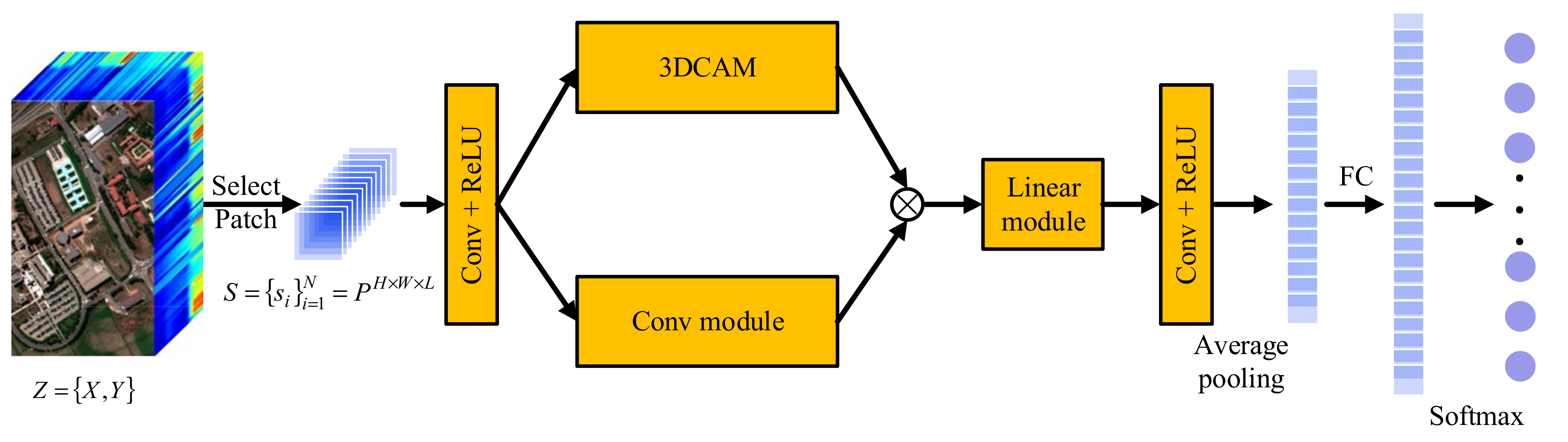
For a hyperspectral image, , where is the set of all pixel data of the image, and is the set of labels corresponding to all pixels. In order to effectively learn edge features, the input image is processed and filled pixel by pixel to obtain cubes with the size . Here, is the space size of the cube, and is the number of spectral bands. The designed 3DCAMNet is mainly composed of three parts. Firstly, the input image is extracted by convolution module. Secondly, in order to fully consider the importance of the space and spectrum of the input image, a 3D coordination attention mechanism (3DCAM) is designed. After feature extraction, in order to extract advanced features more accurately, inspired by the ghost module, a linear module is designed. Lastly, the final classification results are obtained through the full connection layer (FC) and softmax layer. The overall framework of 3DCAMNet is shown in Figure 1. Next, we introduce the principle and framework of each module in 3DCAMNet step by step.
2.2. DCAM
Application of the attention mechanism in a convolutional neural network (CNN) can effectively enhance the ability of feature discrimination, and it is widely used in hyperspectral image classification. Hyperspectral images contain rich spatial and spectral information. However, in feature extraction, effectively extracting spatial and spectral dimensional features is the key to better classification. Therefore, we propose a 3D coordination attention mechanism (3DCAM), which is used to explore the long-distance relationship between the vertical and horizontal directions of spatial dimension and the difference of band importance of spectral dimension. The attention mechanism obtains the attention masks of the spatial dimension and spectral dimension according to the long-distance relationship between the vertical and horizontal directions of spatial information and the difference of importance of spectral information.
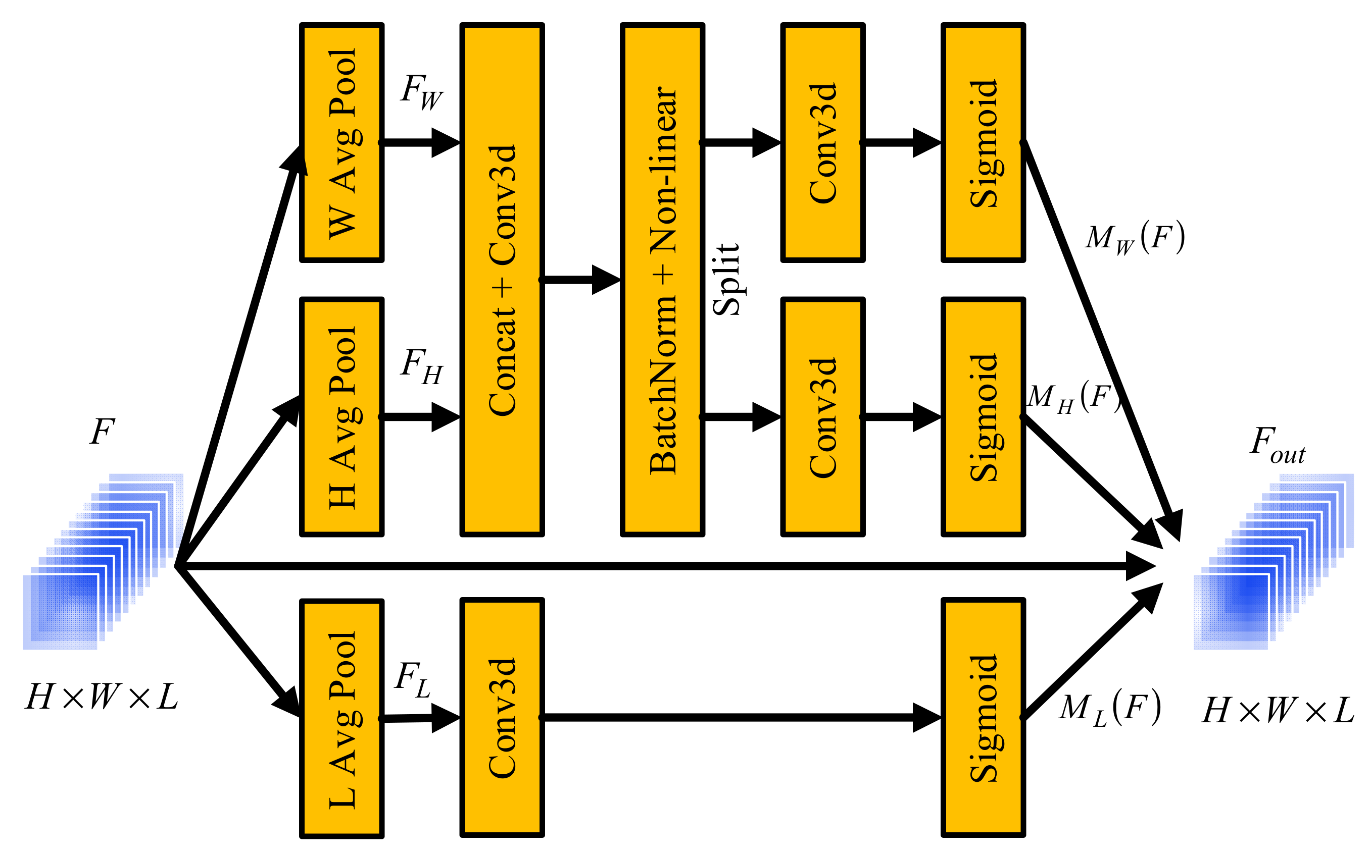
The structure of the proposed 3DCAM is shown in Figure 2. 3DCAM includes two parts (spectral attention and spatial coordination attention). Spectral and spatial attention can adaptively learn different spectral bands and spatial backgrounds, so as to improve the ability to distinguish different bands and obtain more accurate spatial relationships. Assuming that the input of 3DCAM is , the output can be represented as
where and represent the input and output of 3DCAM, respectively. represents the attention map in direction , and the output size is . represents the attention map in direction , and the output size is . Similarly, represents the attention map in direction , and the output size is . and are obtained by considering the vertical and horizontal directions of spatial information, so as to obtain long-distance dependent information. Specifically, obtains in the vertical direction and in the horizontal direction through the global average pooling layer, and the obtained results are cascaded. In order to obtain the long-distance dependence in the vertical and horizontal directions, the cascaded results are sent to the unit convolution layer, batch normalization layer (BN), and nonlinear activation layer. The activation function of the nonlinear activation layer is h_swish [58], this kind of activation function has relatively few parameters, which results in the neural network having richer representation ability. The h_swish function can be expressed as
where is a trainable parameter. Finally, the obtained results are separated and convoluted to obtain the vertical attention map and the horizontal attention map .
Similarly, passes through the global average pool layer to obtain , and then the obtained result passes through the unit convolution layer and the activation function layer to obtain the spectral attention map . The implementation process of 3DCAM is shown in Algorithm 1.
| Algorithm 1 Details of 3DCAM. |
| 1: Input: |
| 2: Features: . |
| 3: Output: |
| 4: Feature of 3DCAM: . |
| 5: Initialzation: |
| 6: Initialize all weight parameters of convolutional kernels. |
| 7: passes through Avgpool, AvgPool, and AvgPool layers to generate , , and |
| 8: , respectively; |
| 9: Reshape the size of feature to 1 × H × 1 and cascade with to generate ; |
| 10: Convolute with the 3D unit convolution kernel and the results through regularization and nonlinear a: |
| 11: tivation function layer to generate ; |
| 12: Split and convolute the results with 3D unit convolution kernel to generate and ; |
| 13: Normalize and with the sigmoid function to generate the attention features and |
| 14: ; |
| 15: Convolute with the 3D unit convolution kernel to generate ; |
| 16: Normalize with the sigmoid function to generate the attention feature ; |
| 17: Finally, the attention features ,, and are added to the input feature to |
| 18: obtain . |
2.3. Convolution Module
CNNs have strong feature extraction abilities. In particular, it is possible to use the convolution and pooling operations in a CNN to get deeper information from input data. Due to the data properties of HSIs, the application of a three-dimensional convolutional neural network (3DCNN) can preserve the correlation between data pixels, so that the data will not be lost. In addition, the effective extraction of spatial and spectral information in hyperspectral images is still the focus of hyperspectral image classification.
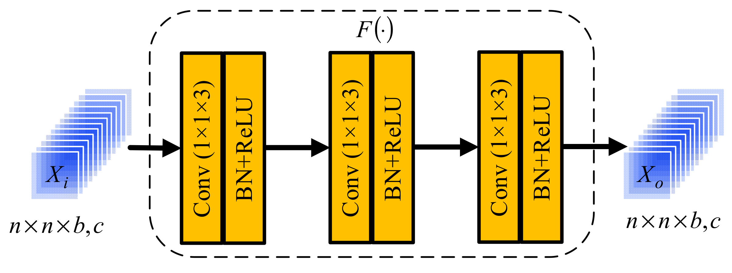
In order to effectively extract the spatial–spectral features of HSIs, a convolution block based on space and spectrum is proposed in this paper. Inspired by Inception V3 [58], the convolution layer uses a smaller convolution kernel, which can not only learn the spatial–spectral features of HSIs, but also effectively reduce the parameters. The structure of the convolution module based on space and spectrum is shown in Figure 3.
As can be seen from Figure 3, input consists of feature maps with the size of . is the output of input after multilayer convolution, which can be expressed as
where is a nonlinear composite function. Specifically, the neural network consists of three layers, and each layer is composed of a convolution, batch normalization (BN), and nonlinear activation function (ReLU). The convolution kernel size of the convolution layer is 1 × 1 × 3. The use of the ReLU function can increase the nonlinear relationship between various layers of neural network, and then complete the complex tasks of neural network, as shown below.
where represents the input of the nonlinear activation function, and represents the nonlinear activation function.
In addition, in order to accelerate the convergence speed, BN layer is added before ReLU to normalize the data, which alleviates the problem of gradient dispersion to a certain extent [59]. The normalization formula is as follows:
where represents the average input value of each neuron, and represents the standard deviation of the input value of each neuron.
2.4. Linear Module
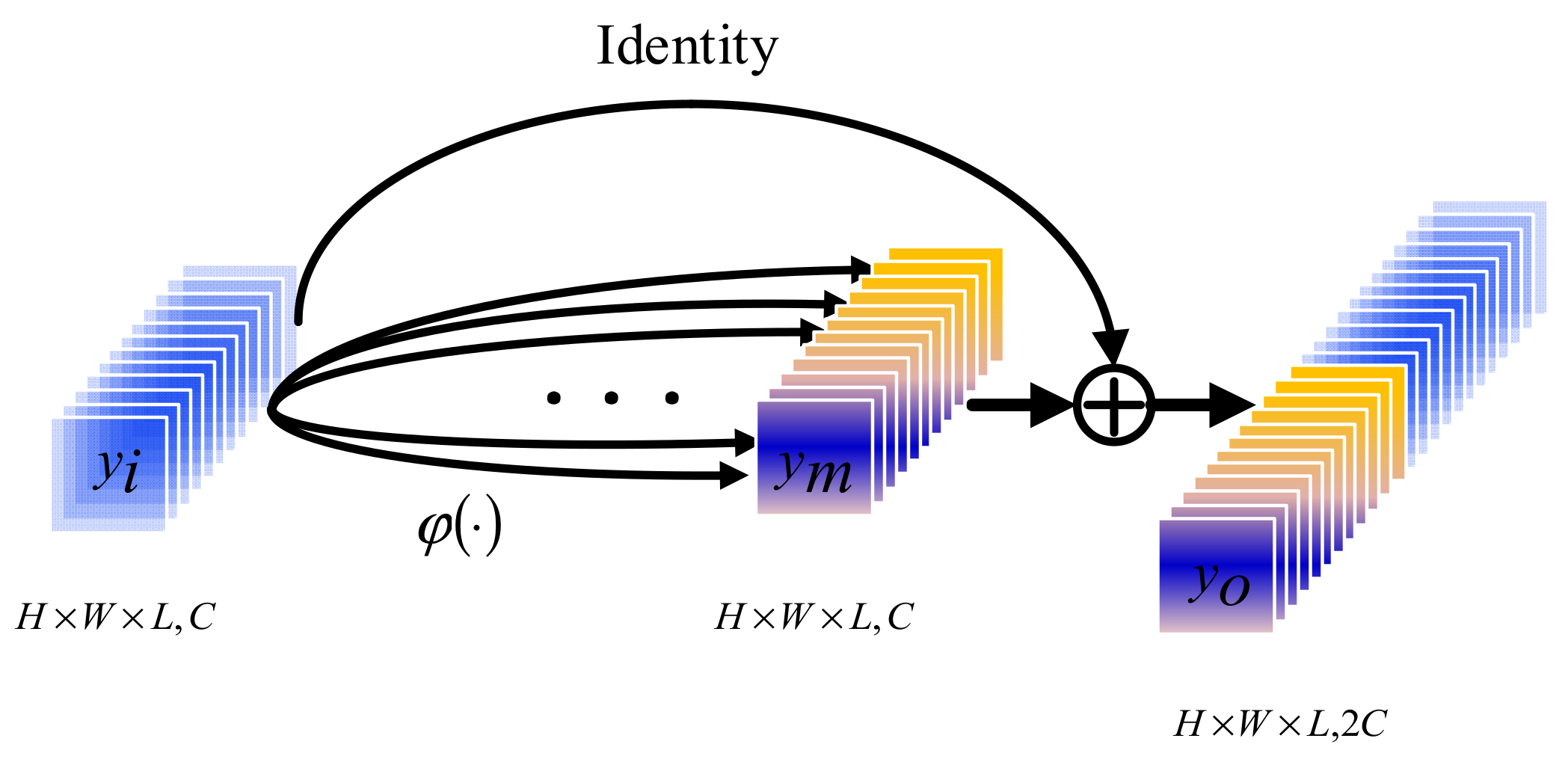
In the task of hyperspectral image classification, extracting feature information as much as possible is the key to improve the classification performance. Inspired by the ghost module [60], this paper adopts a linear module. On the basis of the features output after the fusion of 3DCAM and convolution module, the feature map containing more information is generated by linear module.
The structure of the linear module is shown in Figure 4. The input is linearly convoluted to obtain , and then the obtained feature map is cascaded with the input to obtain the output . The output of linear convolution is calculated as follows:
where is a linear convolution function, represents the neuron at the position of the -th feature map on the -th layer, , and represent the height, width, and spectral dimension of the convolution kernel, respectively, and is the index of feature map. In addition, represents the weight of the -th convolution kernel on at the -th feature map position of layer . represents the value of the neuron at of the -th feature map on layer , and is the bias term.
3. Experimental Results and Analysis
In order to verify the classification performance of 3DCAMNet, this section conducts a series of experiments using five datasets. All experiments are implemented on the same configuration, i.e., an Intel (R) core (TM) i9-9900k CPU, NVIDIA Geforce RTX 2080TI GPU, and 32 GB random access memory server. The contents of this section include the experimental setup, comparison of results, and discussion.
3.1. Experimental Setting
3.1.1. Datasets
Five common datasets were selected, namely, Indian Pines (IP), Pavia University (UP), Kennedy Space Center (KSC), Salinas Valley (SV), and University of Houston (HT). The IP, KSC, and SV datasets were captured by airborne visible infrared imaging spectrometer (AVIRIS) sensors. The UP and HT datasets were obtained by the reflective optical spectral imaging system (ROSIS-3) sensor and the compact airborne spectral imager (CASI) sensor, respectively.
Specifically, IP has 16 feature categories with a space size of 145 × 145, and 200 spectral bands can be used for experiments. Compared with IP, UP has fewer feature categories, only nine, and the image size is 610 × 340. In addition to 13 noise bands, 103 bands are used in the experiment. The spatial resolution of KSC is 20 m and the spatial size of each image is 512 × 614. Similarly, after removing the water absorption band, 176 bands are left for the experiment. The SV space size is 512 × 217 and contains 16 feature categories, while there are 204 spectral bands available for experiments. The last dataset HT has a high spatial resolution and a spatial size of 349 × 1905, the number of bands is 114, and the wavelength range is 380–1050 nm, including 15 feature categories. The details of the dataset are shown in Table 1.
3.1.2. Experimental Setting
In 3DCAMNet, the batch size and maximum training rounds used were 16 and 200, respectively, and the “Adam” optimizer was selected during the training process. The learning rate and input space size were 0.0005 and 9 × 9, respectively. In addition, the cross-loss entropy was used to measure the difference between the real probability distribution and the predicted probability distribution. Table 2 shows the superparameter settings of 3DCAMNet.
3.1.3. Evaluation Index
Three evaluation indicators were adopted in the experiments, namely, overall accuracy (OA), average accuracy (AA), and Kappa coefficient (Kappa) [61]. The measuremnet units of these evaluation indicators are all dimensionless. The confusion matrix is constructed with the real category information of the original pixel and the predicted category information, where is the number of categories, and is the number of samples classified as category by category . Assuming that the total number of samples of HSIs is , the ratio of the number of accurately classified samples to the total number of samples OA is
where, is the correctly classified element in the confusion matrix. Similarly, AA is the average value of classification accuracy for each category,
The Kappa matrix is another performance evaluation index. The specific calculation is as follows:
where and represent all column elements in row and all row elements in column of confusion matrix , respectively.
3.2. Experimental Results
In this section, the proposed method 3DCAMNet is compared with other advanced classification methods, including SVM [17], SSRN [52], PyResNet [40], DBMA [53], DBDA [55], Hybrid-SN [35], and A2S2K-ResNet [57]. In the experiment, the training proportion of IP, UP, KSC, SV, and HT datasets was 3%, 0.5%, 5%, 0.5%, and 5%. In addition, for fair comparison, the input space size of all methods was 9 × 9, and the final experimental results were the average of 30 experiments.
SVM is a classification method based on the radial basis kernel function (RBF). SSRN designs a residual module of space and spectrum to extract spatial–spectral information for the neighborhood blocks of input three-dimensional cube data. PyResNet gradually increases the feature dimension of each layer through the residual method, so as to get more location information. In order to further improve the classification performance, DBMA and DBDA designed spectral and spatial branches to extract the spectral–spatial features of HSIs, respectively, and used an attention mechanism to emphasize the channel features and spatial features in the two branches, respectively. Hybrid-SN verifies the effectiveness of a hybrid spectral CNN network, whereby spectral–spatial features are first extracted through 3DCNN, and then spatial features are extracted through 2DCNN. A2S2K-ResNet designs an adaptive kernel attention module, which not only solves the problem of automatically adjusting the receptive fields (RFs) of the network, but also jointly extracts spectral–spatial features, so as to enhance the robustness of hyperspectral image classification. Unlike the attention mechanism proposed in the above methods, in order to obtain the long-distance dependence in the vertical and horizontal directions and the importance of the spectrum, a 3D coordination attention mechanism is proposed in this paper. Similarly, in order to further extract spectral and spatial features with more discriminant features, the 3DCNN and linear module are used to fully extract joint spectral–spatial features, so as to improve the classification performance.
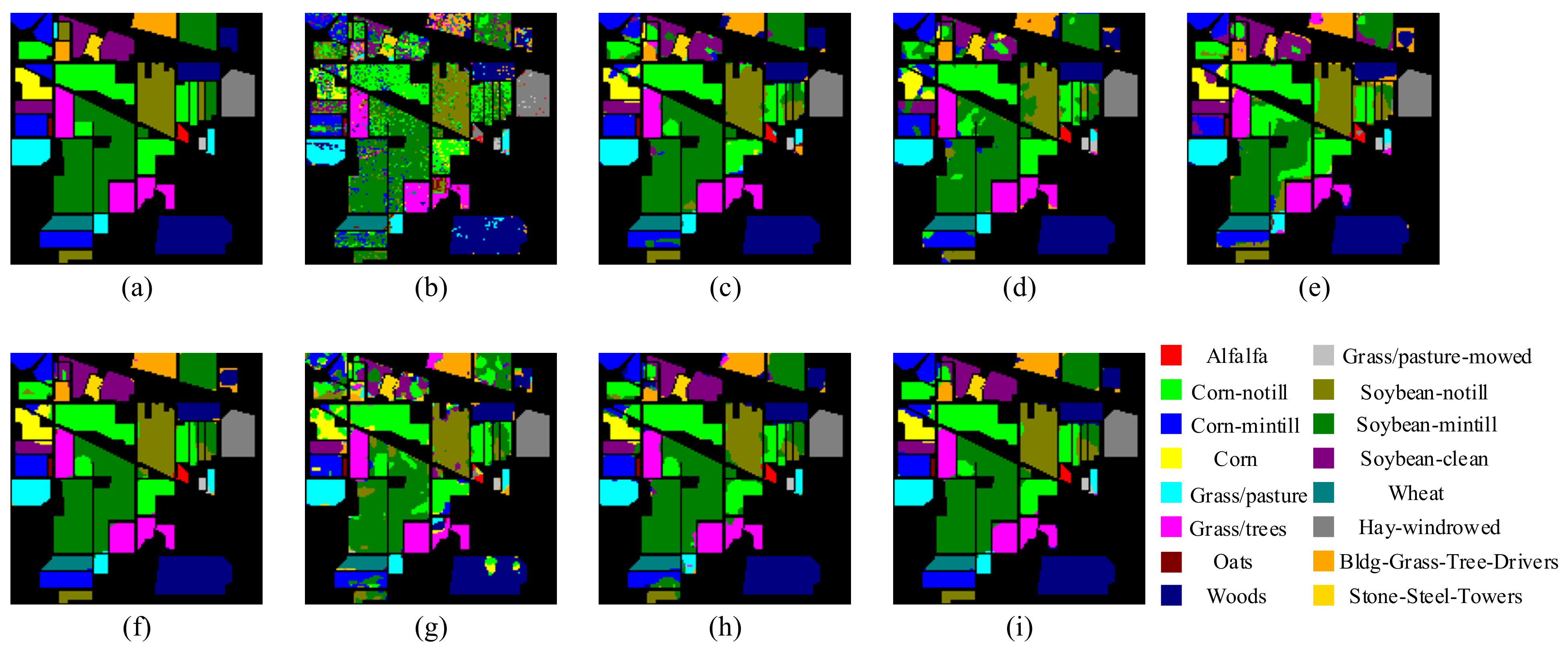
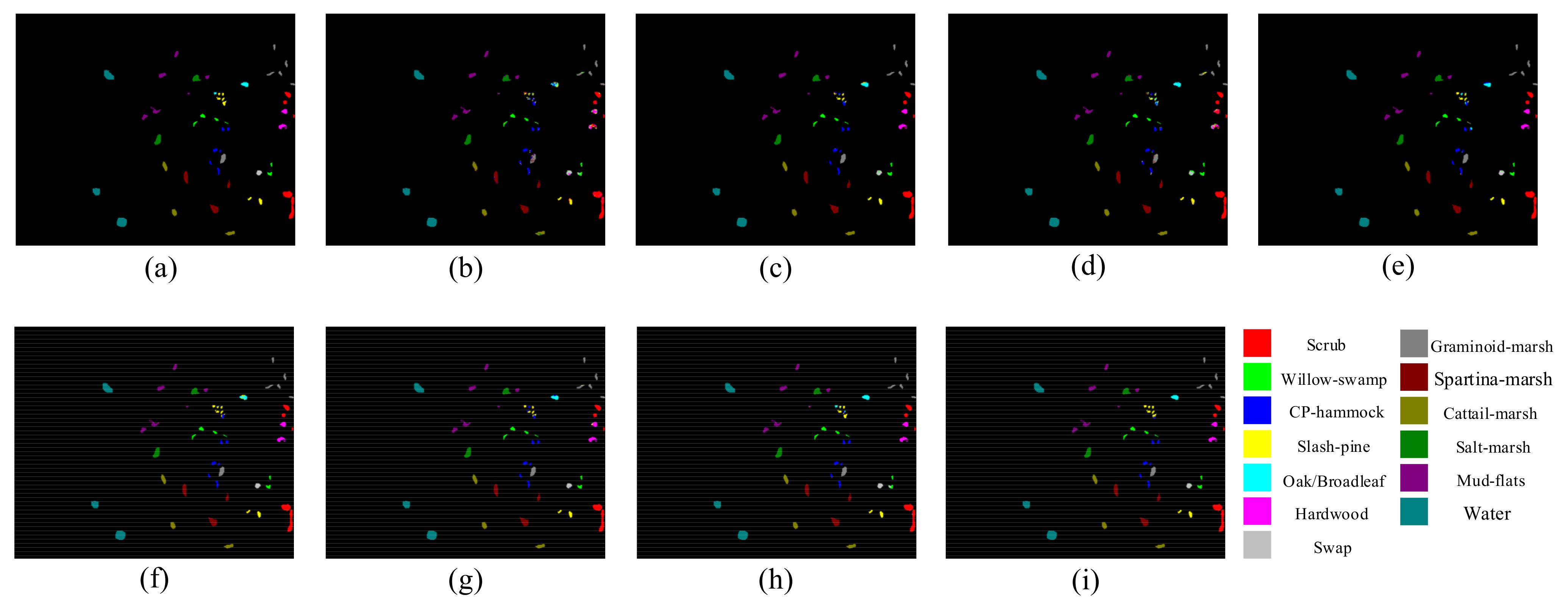
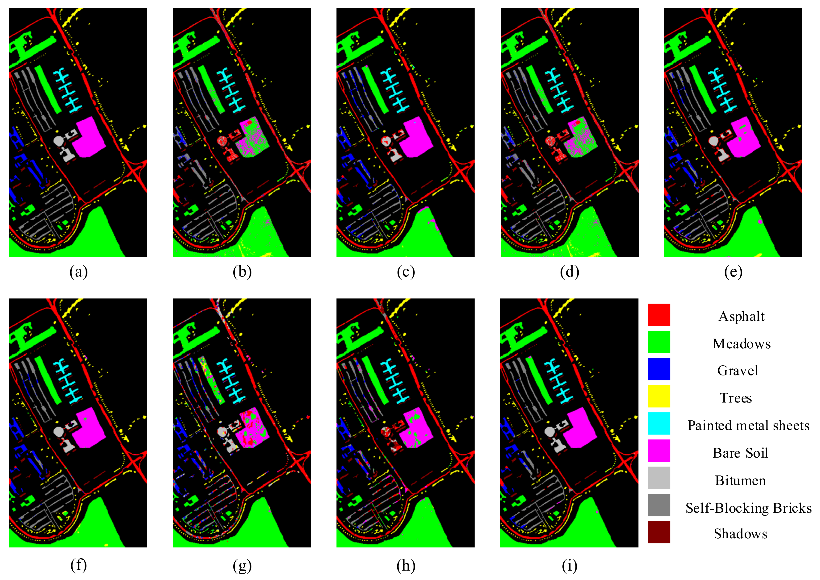
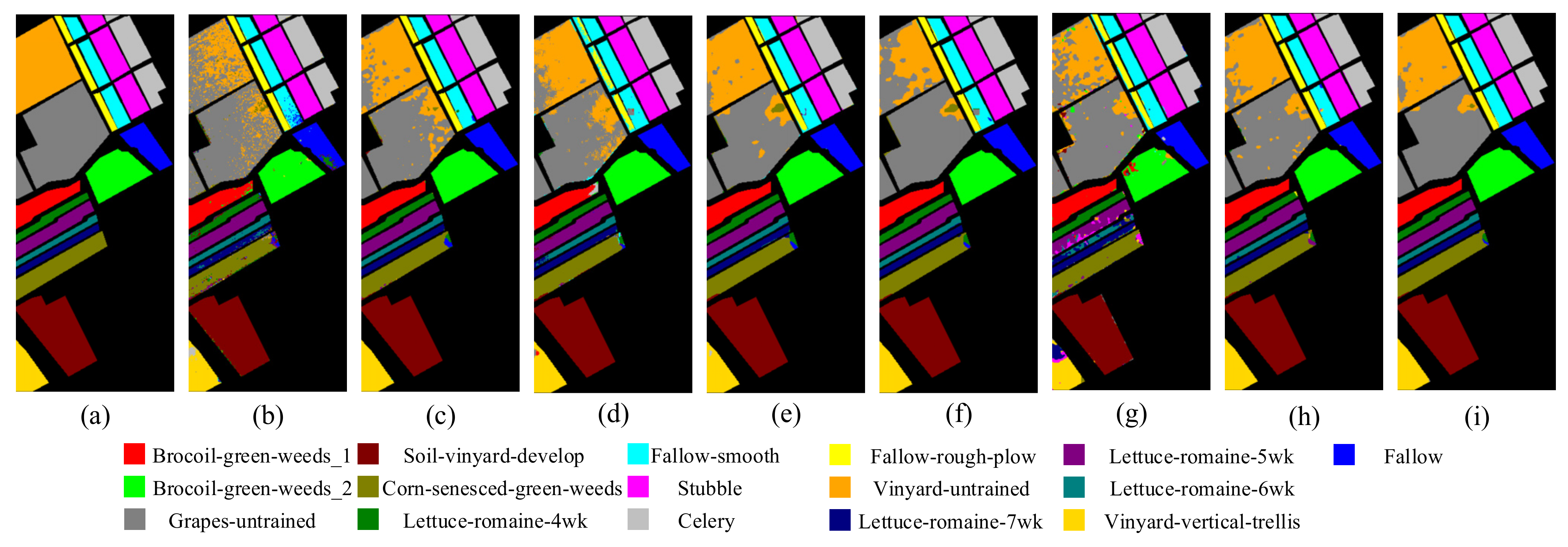
The classification accuracy of all methods on IP, UP, KSC, SV, and HT datasets are show in Table A1, Table A2, Table A3, Table A4 and Table A5, respectively. It can be seen that, in the five datasets, compared with other methods, the method proposed in this paper not only obtained the best OA, AA, and Kappa, but also almost every class had greater advantages in classification accuracy. Specifically, due to the complex distribution of features in the IP dataset, the classification accuracy of all methods on this dataset was low, but the method in this paper not only obtained better accuracy in the categories that were easy to classify, but also obtained better accuracy in the categories that were difficult to classify such as Class 2, Class 4, and Class 9. Similarly, in the UP dataset, we can clearly see that the accuracy of the method proposed in this paper, according to OA, AA, and Kappa or various categories, has great advantages over other methods. Compared with the IP dataset, the UP dataset has fewer feature categories, and all methods exhibited better classification results, but the method in this paper obtained the highest classification accuracy. The KSC dataset has the same number of categories as the IP dataset, in addition to 16 feature categories, but the KSC feature categories are scattered. It can be seen from Table A3 that all classification methods obtained ideal results, but the proposed method obtained the best classification accuracy. In addition, because the sample distribution of the SV dataset is relatively balanced and the ground object distribution is relatively regular, the classification accuracy of all methods was high. On the contrary, HT images were collected from the University of Houston Campus, with complex distribution and many categories, but the method proposed in this paper could still achieve high-precision classification.
In addition, Figure 5, Figure 6, Figure 7, Figure 8 and Figure 9 shows the classification visualization results of all methods, including the false-color composite image and the classification visualization results of each method. Because the traditional classification methods cannot effectively extract spatial–spectral features, the classification effect was poor, while the image was rough and noisy, as seen for SVM and the deep network methods based on ResNet, including SSRN and PyResNet. Although these kinds of method can obtain good classification results, there was still a small amount of noise. In addition, DBMA, DBDA, and A2S2K-ResNet all added an attention mechanism to the network, which yielded better classification visualization results, but there were still many classification errors. However, the classification visualization results obtained by the method proposed in this paper were smoother and closer to the real feature map. This fully verifies the superiority of the proposed method.
In conclusion, through multiple angle analysis, it was verified that this method has more advantages than other methods. First, among all methods, the proposed method had the highest overall accuracy (OA), average accuracy (OA), and Kappa coefficient (Kappa). In addition, the method proposed in this paper could not only achieve high classification accuracy in the categories that were easy to classify, but also had strong judgment ability in the categories that were difficult to classify. Second, among the classification visualization results of all methods, the method in this paper obtained smoother results that were closer to the false-color composite image.
4. Discussion
In this section, we discuss in detail the modules and parameters that affect the classification performance of the proposed method, including the impact of different attention mechanisms on classification accuracy OA, the impact of different input space sizes and different training sample ratios on classification accuracy OA, ablation experiments of different modules in 3DCAMNet, and the comparison of running time and parameters of different methods on IP datasets.
4.1. Effects of Different Attention Mechanisms on OA
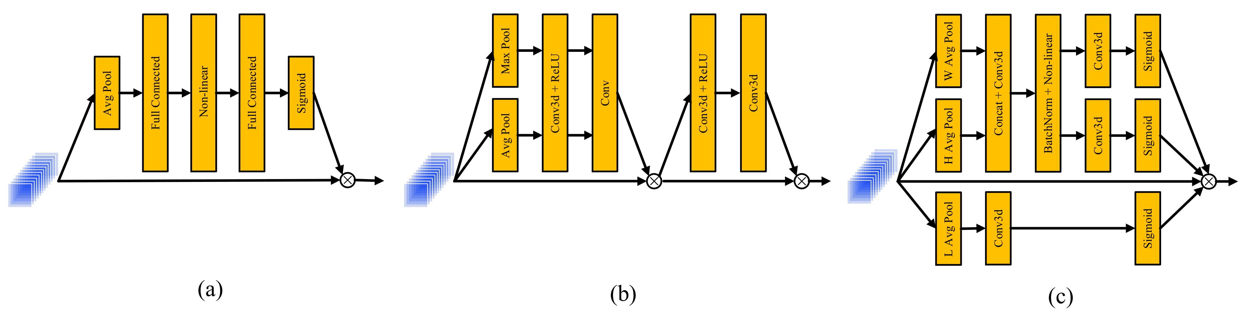
In order to verify the effectiveness of 3DCAM, we consider two other typical attention mechanisms for comparison, SE and CBAM, as shown in Figure 10. The experimental results of the three attention mechanisms are shown in Table 3. The results show that the classification accuracy of 3DCAM on the five datasets was better than SE and CBAM, and the attention mechanism of CBAM was better than SE on a whole. The reason is that SE attention only emphasizes the importance differences of channels, without considering spatial differences. Although CBAM considers the channel dependence and spatial dependence, it does not fully consider the spatial location information. Lastly, for hyperspectral data types, 3DCAM fully considers the position relationship in the horizontal and vertical directions of space, obtains the long-distance dependence, and considers the differences in spectral dimension. Therefore, our proposed 3DCAM can better mark important spectral bands and spatial location information.
4.2. Effects of Different Input Space Sizes and Different Training Sample Ratios on OA
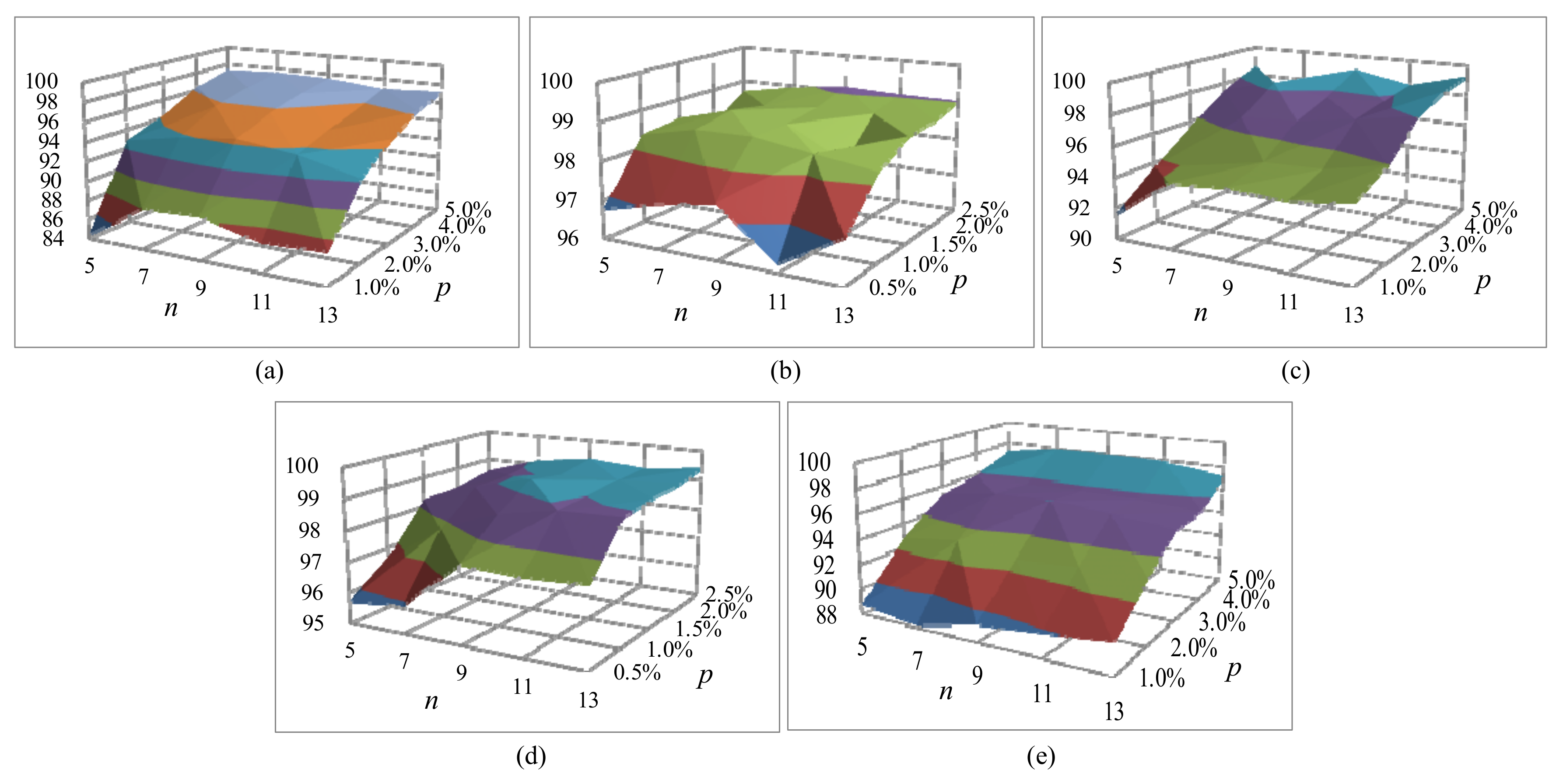
The size of input space and the proportion of different training samples are two important superparameters of 3DCAMNet, and their changes have a great impact on the classification performance. In particular, the selected input space sizes of 5 × 5, 7 × 7, 9 × 9, 11 × 11, and 13 × 13 were used to explore the optimal space size of 3DCAMNet method. In addition, the proportion of training samples refers to the proportion of training samples used by the network. Among them, the value of for the IP, KSC, and HT datasets was , while the value of for the UP and SV datasets was . Figure 11 shows the OA results of 3DCAMNet with different input size n and different training sample ratio for all datasets. As can be seen from Figure 11, when and the proportion of training samples of IP, UP, KSC, SV, and HT datasets was 1.0%, 0.5%, 1.0%, 0.5%, and 1.0%, respectively, the OA value obtained by the proposed method was the lowest. With the increase in proportion of training samples, OA increased slowly. In addition, when and the number of training samples was the highest, the classification performance obtained better results.
4.3. Comparison of Contributions of Different Modules in 3DCAMNet
In order to verify the effectiveness of the method proposed in this paper, we conducted ablation experiments on two important modules of the method: the linear module and 3DCAM. The experimental results are shown in Table 4. It can be seen that, when both the linear module and 3DCAM were implemented, the OA value obtained on all datasets was the largest, which fully reflects the strong generalization ability of the proposed method. On the contrary, when neither module was implemented, the OA value obtained on all datasets was the lowest. In addition, when either the linear module or the 3DCAM module was applied to the network, the overall accuracy OA was improved. In general, the ablation experiment shows that the classification performance of the basic network was the lowest, but with the gradual addition of modules, the classification performance was also gradually improved. The ablation experiments fully verified the effectiveness of the linear module and 3DCAM.
4.4. Comparison of Running Time and Parameters of Different Methods on IP Dataset
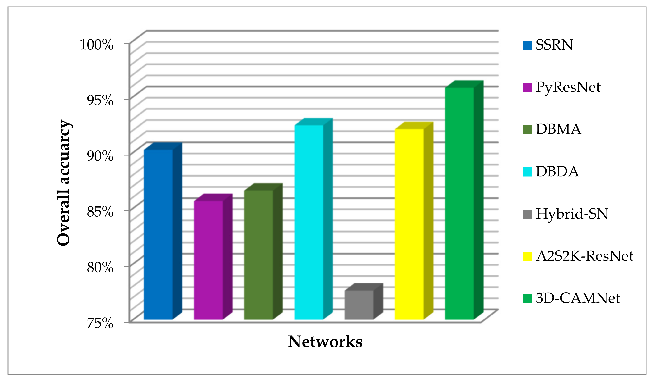
When the input size was 9 × 9 × 200, the comparison results of parameter quantity and running time between 3DCAMNet and other advanced methods were as shown in Table 5. It can be seen that the PyResNet based on space and spectrum needed the most parameters. This is because it obtains more location information by gradually increasing the feature dimension of all layers, which inevitably necessitates more parameters. In addition, the longest running time of all methods was DBDA. However, the parameter amount of the proposed method was similar to that of other methods, and the running time was also moderate. For further comparison, the OA values obtained by these methods on the IP dataset are shown in Figure 12. Combined with Table 5, it can be seen that, compared with other methods, the parameter quantity and running time of the proposed 3DCAMNet were moderate, while 3DCAMNet method could achieve the highest OA.
5. Conclusions
A 3DCAMNet method was proposed in this paper. It is mainly composed of three modules: a convolution module, linear module, and 3DCAM. Firstly, the convolution module uses 3DCNN to fully extract spatial–spectral features. Secondly, the linear module is introduced after the convolution module to extract more fine features. Lastly, 3DCAM was designed, which can not only obtain the long-distance dependence between vertical and horizontal directions in HSI space, but also obtain the importance difference between different spectral bands. The proposed 3DCAM was compared with two classical attention mechanisms, i.e., SE and CBAM. The experimental results show that the classification method based on 3DCAM could obtain better classification performance. Compared with some state-of-the art methods, such as A2S2K-ResNet and Hybrid-SN, 3DCAMNet could achieve better classification performance. The reason is that, although A2S2K-ResNet can expand the receptive field (RF) via the adaptive convolution kernel, the deep features cannot be reused. Similarly, Hybrid-SN can extract spatial and spectral features using 2DCNN and 3DCNN, but the classification performance was still worse than that of 3DCAMNet because of its small RF and insufficient extracted features. In addition, in order to verify the effectiveness of the proposed method, a series of experiments were carried out on five datasets. The experimental results show that 3DCAMNet had higher classification performance and stronger robustness than other state-of-the-art methods, highlighting the effectiveness of the proposed 3DCAMNet method in hyperspectral classification. In future work, we will consider a more efficient attention mechanism module and spatial–spectral feature extraction module.
Author Contributions
Conceptualization, C.S. and D.L.; data curation, D.L.; formal analysis, T.Z.; methodology, C.S. and D.L.; software, D.L.; validation, D.L. and C.S.; writing—original draft, D.L.; writing—review and editing, C.S. and L.W. All authors have read and agreed to the published version of the manuscript.
Funding
This research was funded in part by the Heilongjiang Science Foundation Project of China under Grant LH2021D022, in part by the National Natural Science Foundation of China (41701479, 62071084), and in part by the Fundamental Research Funds in Heilongjiang Provincial Universities of China under Grant 135509136.
Institutional Review Board Statement
Not applicable.
Informed Consent Statement
Not applicable.
Data Availability Statement
Data associated with this research are available online. The IP dataset is available for download at http://www.ehu.eus/ccwintco/index.php/Hyperspectral_Remote_Sensing_Scenes (accessed on 21 November 2021). The UP dataset is available for download at http://www.ehu.eus/ccwintco/index.php/Hyperspectral_Remote_Sensing_Scenes#Pavia_University_scene (accessed on 21 November 2021). The KSC dataset is available for download at http://www.ehu.eus/ccwintco/index.php/Hyperspectral_Remote_Sensing_Scenes (accessed on 21 November 2021). The SV dataset is available for download at http://www.ehu.eus/ccwintco/index.php/Hyperspectral_Remote_Sensing_Scenes (accessed on 21 November 2021). The HT dataset is available for download at http://www.grss-ieee.org/community/technical-committees/data-fusion/2013-ieee-grss-data-fusion-contest/ (accessed on 21 November 2021).
Acknowledgments
We would like to thank the handling editor and the anonymous reviewers for their careful reading and helpful remarks.
Conflicts of Interest
The authors declare no conflict of interest.
Appendix A

Table A1.
Classification results of different methods on IP dataset (%).
| Class | SVM [17] | SSRN [52] | PyResNet [40] | DBMA [53] | DBDA [55] | Hybrid-SN [35] | A2S2K-ResNet [57] | Proposed |
|---|---|---|---|---|---|---|---|---|
| 1 | 36.62 | 87.22 | 26.67 | 82.90 | 87.99 | 73.05 | 89.41 | 98.78 |
| 2 | 55.49 | 85.71 | 80.92 | 82.84 | 90.61 | 66.14 | 90.49 | 96.38 |
| 3 | 62.33 | 90.65 | 81.24 | 79.53 | 92.07 | 77.63 | 92.32 | 94.80 |
| 4 | 42.54 | 83.86 | 62.17 | 87.42 | 93.96 | 62.61 | 93.78 | 94.98 |
| 5 | 85.05 | 98.41 | 91.75 | 96.36 | 99.02 | 89.56 | 97.83 | 98.89 |
| 6 | 83.32 | 98.29 | 94.26 | 96.62 | 96.82 | 92.23 | 97.20 | 98.11 |
| 7 | 59.87 | 82.98 | 19.75 | 49.28 | 67.63 | 44.90 | 88.70 | 70.53 |
| 8 | 89.67 | 97.81 | 100.00 | 99.14 | 98.94 | 90.65 | 98.81 | 100.00 |
| 9 | 39.28 | 67.03 | 69.09 | 54.77 | 78.24 | 37.79 | 64.56 | 92.71 |
| 10 | 92.32 | 88.23 | 82.96 | 83.92 | 84.03 | 70.23 | 88.59 | 91.24 |
| 11 | 64.73 | 89.39 | 89.59 | 90.97 | 93.92 | 77.38 | 89.76 | 96.67 |
| 12 | 50.55 | 86.98 | 59.82 | 80.15 | 88.91 | 67.60 | 92.48 | 92.01 |
| 13 | 86.74 | 99.06 | 80.07 | 97.46 | 97.81 | 82.10 | 96.89 | 99.58 |
| 14 | 88.67 | 97.16 | 96.31 | 95.68 | 97.63 | 93.12 | 96.02 | 97.51 |
| 15 | 61.82 | 82.01 | 86.36 | 82.46 | 91.48 | 76.21 | 91.34 | 94.31 |
| 16 | 98.66 | 96.30 | 90.37 | 94.50 | 89.81 | 45.12 | 93.31 | 97.29 |
| OA (%) | 68.76 | 90.24 | 85.65 | 86.59 | 92.44 | 77.61 | 92.10 | 95.81 |
| AA (%) | 66.73 | 89.44 | 75.67 | 84.63 | 90.55 | 71.65 | 91.36 | 94.61 |
| Kappa (%) | 63.98 | 88.86 | 83.6 | 84.79 | 91.38 | 74.35 | 90.97 | 95.22 |
Table A2.
Classification results of different methods on UP dataset (%).
| Class | SVM [17] | SSRN [52] | PyResNet [40] | DBMA [53] | DBDA [55] | Hybrid-SN [38] | A2S2K-ResNet [57] | Proposed |
|---|---|---|---|---|---|---|---|---|
| 1 | 81.26 | 94.60 | 88.11 | 92.22 | 94.24 | 74.67 | 83.81 | 95.57 |
| 2 | 84.53 | 98.15 | 97.77 | 96.34 | 99.16 | 92.08 | 92.72 | 99.38 |
| 3 | 56.56 | 74.38 | 30.97 | 83.79 | 91.03 | 63.00 | 72.97 | 92.63 |
| 4 | 94.34 | 96.11 | 84.79 | 95.92 | 97.01 | 83.44 | 98.12 | 97.77 |
| 5 | 95.38 | 98.94 | 96.64 | 98.85 | 98.83 | 88.95 | 98.68 | 98.74 |
| 6 | 80.66 | 92.09 | 54.3 | 91.58 | 98.27 | 83.42 | 86.51 | 98.45 |
| 7 | 94.13 | 69.86 | 38.3 | 88.04 | 98.48 | 68.86 | 88.07 | 99.66 |
| 8 | 71.12 | 84.54 | 75.5 | 81.64 | 88.38 | 56.96 | 74.11 | 87.19 |
| 9 | 99.94 | 88.86 | 91.15 | 93.22 | 97.98 | 65.31 | 90.97 | 98.87 |
| OA (%) | 82.06 | 92.76 | 83.01 | 92.32 | 96.52 | 81.33 | 87.45 | 97.01 |
| AA (%) | 79.22 | 88.61 | 73.06 | 91.29 | 95.93 | 75.19 | 87.33 | 96.47 |
| Kappa (%) | 75.44 | 90.43 | 76.9 | 89.79 | 95.37 | 75.01 | 83.16 | 96.02 |
Table A3.
Classification results of different methods on KSC dataset (%).
| Class | SVM [17] | SSRN [52] | PyResNet [40] | DBMA [53] | DBDA [55] | Hybrid-SN [38] | A2S2K-ResNet [57] | Proposed |
|---|---|---|---|---|---|---|---|---|
| 1 | 92.43 | 97.88 | 94.10 | 100.00 | 100.00 | 99.41 | 100.00 | 99.82 |
| 2 | 87.14 | 92.67 | 85.59 | 93.38 | 96.17 | 93.25 | 99.13 | 97.61 |
| 3 | 72.47 | 86.11 | 81.15 | 80.70 | 91.28 | 86.45 | 87.81 | 98.94 |
| 4 | 54.45 | 86.50 | 77.23 | 68.91 | 83.62 | 93.34 | 98.53 | 92.40 |
| 5 | 64.11 | 74.79 | 74.97 | 74.41 | 79.30 | 93.86 | 92.36 | 95.94 |
| 6 | 65.23 | 99.05 | 78.77 | 95.51 | 96.11 | 95.72 | 99.92 | 99.53 |
| 7 | 75.50 | 84.92 | 84.74 | 85.81 | 94.89 | 94.94 | 95.85 | 96.97 |
| 8 | 87.33 | 98.48 | 95.22 | 94.93 | 98.90 | 97.75 | 99.41 | 99.97 |
| 9 | 87.94 | 98.47 | 93.94 | 96.81 | 99.98 | 98.94 | 99.76 | 99.98 |
| 10 | 97.01 | 99.21 | 98.97 | 99.27 | 100.00 | 99.97 | 100.00 | 100.00 |
| 11 | 96.03 | 99.23 | 99.48 | 99.59 | 99.16 | 99.14 | 100.00 | 98.86 |
| 12 | 93.76 | 98.46 | 96.14 | 97.47 | 99.30 | 99.13 | 99.64 | 99.48 |
| 13 | 99.72 | 99.89 | 99.73 | 100.00 | 100.00 | 99.61 | 100.00 | 100.00 |
| OA (%) | 87.96 | 95.42 | 91.49 | 94.15 | 97.33 | 97.32 | 98.34 | 99.01 |
| AA (%) | 82.55 | 93.51 | 89.23 | 91.29 | 95.28 | 96.27 | 97.87 | 98.42 |
| Kappa (%) | 86.59 | 94.91 | 90.52 | 93.48 | 97.02 | 97.02 | 98.84 | 98.88 |
Table A4.
Classification results of different methods on SV dataset (%).
| SV | SVM [17] | SSRN [52] | PyResNet [40] | DBMA [53] | DBDA [55] | Hybrid-SN [38] | A2S2K-ResNet [57] | Proposed |
|---|---|---|---|---|---|---|---|---|
| 1 | 99.42 | 96.56 | 98.49 | 100.00 | 99.62 | 96.70 | 99.84 | 100.00 |
| 2 | 98.79 | 99.72 | 99.69 | 99.98 | 99.25 | 97.11 | 99.99 | 99.95 |
| 3 | 87.98 | 93.64 | 96.37 | 97.43 | 96.85 | 95.83 | 94.98 | 97.80 |
| 4 | 97.54 | 97.29 | 96.69 | 93.46 | 94.34 | 53.87 | 96.16 | 97.06 |
| 5 | 95.10 | 94.47 | 91.03 | 98.70 | 95.42 | 90.34 | 99.13 | 98.92 |
| 6 | 99.90 | 99.74 | 99.61 | 98.86 | 99.99 | 97.03 | 99.73 | 99.96 |
| 7 | 95.59 | 98.86 | 98.69 | 97.98 | 98.58 | 98.35 | 99.72 | 99.89 |
| 8 | 71.66 | 88.73 | 83.09 | 91.98 | 86.80 | 85.17 | 90.15 | 95.84 |
| 9 | 98.08 | 99.52 | 98.86 | 98.62 | 98.99 | 97.93 | 99.67 | 99.67 |
| 10 | 85.39 | 97.05 | 97.55 | 96.95 | 97.62 | 94.65 | 98.52 | 99.10 |
| 11 | 86.98 | 94.69 | 95.31 | 92.83 | 94.28 | 59.18 | 95.21 | 96.43 |
| 12 | 94.20 | 98.15 | 98.19 | 98.63 | 97.95 | 93.87 | 97.64 | 99.79 |
| 13 | 93.43 | 97.86 | 75.11 | 98.51 | 99.45 | 54.35 | 97.10 | 99.93 |
| 14 | 92.03 | 93.24 | 87.30 | 94.28 | 95.29 | 59.06 | 93.29 | 96.53 |
| 15 | 71.02 | 76.41 | 81.15 | 87.54 | 81.18 | 83.34 | 84.79 | 92.20 |
| 16 | 97.82 | 99.20 | 98.55 | 99.55 | 99.71 | 85.75 | 99.77 | 100.0 |
| OA (%) | 86.98 | 91.12 | 91.52 | 95.22 | 92.32 | 89.10 | 94.59 | 97.48 |
| AA (%) | 91.56 | 95.33 | 93.48 | 96.58 | 95.96 | 83.91 | 96.61 | 98.32 |
| Kappa (%) | 85.45 | 90.15 | 90.54 | 94.67 | 91.44 | 87.85 | 93.98 | 97.19 |
Table A5.
Classification results of different methods on HT dataset (%).
| HT | SVM [17] | SSRN [52] | PyResNet [40] | DBMA [53] | DBDA [55] | Hybrid-SN [38] | A2S2K-ResNet [57] | Proposed |
|---|---|---|---|---|---|---|---|---|
| 1 | 95.99 | 94.63 | 89.05 | 93.13 | 95.55 | 78.34 | 98.51 | 97.37 |
| 2 | 96.97 | 98.82 | 95.92 | 97.10 | 98.14 | 83.13 | 99.38 | 99.39 |
| 3 | 99.56 | 99.95 | 99.95 | 99.91 | 99.97 | 97.15 | 99.98 | 100.00 |
| 4 | 97.94 | 99.00 | 95.86 | 98.34 | 98.10 | 84.55 | 97.81 | 99.67 |
| 5 | 95.58 | 97.07 | 98.66 | 98.24 | 99.88 | 85.82 | 99.42 | 99.13 |
| 6 | 99.54 | 99.93 | 94.24 | 99.20 | 99.66 | 87.66 | 97.89 | 99.86 |
| 7 | 88.55 | 95.07 | 94.99 | 93.29 | 95.52 | 68.43 | 97.35 | 95.32 |
| 8 | 84.14 | 90.59 | 90.42 | 94.12 | 98.04 | 66.54 | 99.05 | 99.36 |
| 9 | 82.56 | 94.90 | 83.48 | 93.20 | 95.22 | 61.04 | 94.08 | 96.06 |
| 10 | 86.82 | 92.43 | 78.95 | 91.38 | 92.78 | 65.34 | 94.81 | 96.11 |
| 11 | 87.94 | 98.71 | 87.87 | 95.24 | 96.27 | 65.41 | 97.25 | 97.99 |
| 12 | 84.29 | 95.34 | 88.31 | 93.20 | 95.28 | 62.86 | 96.82 | 97.21 |
| 13 | 76.40 | 96.93 | 94.41 | 91.53 | 94.69 | 79.14 | 97.09 | 90.59 |
| 14 | 97.29 | 99.18 | 97.95 | 98.76 | 99.92 | 79.85 | 97.65 | 99.24 |
| 15 | 99.37 | 98.68 | 98.60 | 97.99 | 98.06 | 80.77 | 99.16 | 99.02 |
| OA (%) | 90.93 | 96.02 | 90.67 | 94.88 | 96.69 | 73.31 | 97.58 | 97.69 |
| AA (%) | 91.53 | 96.75 | 92.58 | 95.64 | 97.14 | 76.40 | 97.75 | 97.75 |
| Kappa (%) | 90.19 | 95.70 | 89.92 | 94.46 | 96.42 | 71.16 | 97.38 | 97.50 |
References
- Li, C.; Ma, Y.; Mei, X.; Liu, C.; Ma, J. Hyperspectral image classification with robust sparse representation. IEEE Geosci. Remote Sens. Lett. 2016, 13, 641–645. [Google Scholar] [CrossRef]
- Yu, C.; Wang, Y.; Song, M.; Chang, C.-I. Class signature-constrained background-suppressed approach to band selection for classification of hyperspectral images. IEEE Trans. Geosci. Remote Sens. 2019, 57, 14–31. [Google Scholar] [CrossRef]
- Yu, H.; Gao, L.; Li, W.; Du, Q.; Zhang, B. Locality sensitive discriminant analysis for group sparse representation-based hyperspectral imagery classification. IEEE Geosci. Remote Sens. Lett. 2017, 14, 1358–1362. [Google Scholar] [CrossRef]
- Yuen, P.W.; Richardson, M. An introduction to hyperspectral imaging and its application for security, surveillance and target acquisition. Imaging Sci. J. 2010, 58, 241–253. [Google Scholar] [CrossRef]
- Li, H.; Song, Y.; Chen, C.L.P. Hyperspectral image classification based on multiscale spatial information fusion. IEEE Trans. Geosci. Remote Sens. 2017, 55, 5302–5312. [Google Scholar] [CrossRef]
- Gevaert, C.M.; Suomalainen, J.; Tang, J.; Kooistra, L. Generation of spectral–temporal response surfaces by combining multispectral satellite and hyperspectral UAV imagery for precision agriculture applications. IEEE J. Sel. Top. Appl. Earth Observ. Remote Sens. 2015, 8, 3140–3146. [Google Scholar] [CrossRef]
- Van der Meer, F. Analysis of spectral absorption features in hyperspectral imagery. Int. J. Appl. Earth Observ. Geoinf. 2004, 5, 55–68. [Google Scholar] [CrossRef]
- Makki, I.; Younes, R.; Francis, C.; Bianchi, T.; Zucchetti, M. A survey of landmine detection using hyperspectral imaging. ISPRS J. Photogramm. Remote Sens. 2017, 124, 40–53. [Google Scholar] [CrossRef]
- Kang, X.; Li, S.; Benediktsson, J.A. Spectral–spatial hyperspectral image classification with edge-preserving filtering. IEEE Trans. Geosci. Remote Sens. 2014, 52, 2666–2677. [Google Scholar] [CrossRef]
- Fauvel, M.; Benediktsson, J.A.; Chanussot, J.; Sveinsson, J.R. Spectral and spatial classification of hyperspectral data using SVMs and morphological profiles. IEEE Trans. Geosci. Remote Sens. 2008, 46, 3804–3814. [Google Scholar] [CrossRef] [Green Version]
- Li, J.; Huang, X.; Gamba, P.; Bioucas-Dias, J.M.; Zhang, L.; Benediktsson, J.A.; Plaza, A. Multiple feature learning for hyperspectral image classification. IEEE Trans. Geosci. Remote Sens. 2015, 53, 1592–1606. [Google Scholar] [CrossRef] [Green Version]
- Chen, Y.; Nasrabadi, N.M.; Tran, T.D. Hyperspectral image classification via kernel sparse representation. IEEE Trans. Geosci. Remote Sens. 2013, 51, 217–231. [Google Scholar] [CrossRef] [Green Version]
- Li, J.; Khodadadzadeh, M.; Plaza, A.; Jia, X.; Bioucas-Dias, J.M. A discontinuity preserving relaxation scheme for spectral—Spatial hyperspectral image classification. IEEE J. Sel. Top. Appl. Earth Observ. Remote Sens. 2016, 9, 625–639. [Google Scholar] [CrossRef]
- Yu, C.; Xue, B.; Song, M.; Wang, Y.; Li, S.; Chang, C.-I. Iterative target-constrained interference-minimized classifier for hyperspectral classification. IEEE J. Sel. Top. Appl. Earth Observ. Remote Sens. 2018, 11, 1095–1117. [Google Scholar] [CrossRef]
- Jia, X.; Kuo, B.-C.; Crawford, M.M. Feature mining for hyperspectral image classification. Proc. IEEE 2013, 101, 676–697. [Google Scholar] [CrossRef]
- Ghamisi, P.; Benediktsson, J.A.; Ulfarsson, M.O. Spectral spatial classification of hyperspectral images based on hidden Markov random fields. IEEE Trans. Geosci. Remote Sens. 2014, 52, 2565–2574. [Google Scholar] [CrossRef] [Green Version]
- Melgani, F.; Bruzzone, L. Classification of hyperspectral remote sensing images with support vector machines. IEEE Trans. Geosci. Remote Sens. 2004, 42, 1778–1790. [Google Scholar] [CrossRef] [Green Version]
- Li, S.; Song, W.; Fang, L.; Chen, Y.; Ghamisi, P.; Benediktsson, J.A. Deep learning for hyperspectral image classification: An overview. IEEE Trans. Geosci. Remote Sens. 2019, 57, 6690–6709. [Google Scholar] [CrossRef] [Green Version]
- Audebert, N.; le Saux, B.; Lefevre, S. Deep learning for classification of hyperspectral data: A comparative review. IEEE Geosci. Remote Sens. Mag. 2019, 7, 159–173. [Google Scholar] [CrossRef] [Green Version]
- Rasti, B.; Hong, D.; Hang, R.; Ghamisi, P.; Kang, X.; Chanussot, J.; Benediktsson, J.A. Feature Extraction for Hyperspectral Imagery: The Evolution from Shallow to Deep. arXiv 2020, arXiv:2003.02822. [Google Scholar]
- Zhang, K.; Zuo, W.; Zhang, L. FFDNet: Toward a fast and flexible solution for CNN-based image denoising. IEEE Trans. Image Process. 2018, 27, 4608–4622. [Google Scholar] [CrossRef] [Green Version]
- Lu, X.; Zheng, X.; Yuan, Y. Remote sensing scene classification by unsupervised representation learning. IEEE Trans. Geosci. Remote Sens. 2017, 55, 5148–5157. [Google Scholar] [CrossRef]
- Ma, X.; Wang, H.; Geng, J. Spectral-spatial classification of hyperspectral image based on deep auto-encoder. IEEE J. Sel. Top. Appl. Earth Observ. Remote Sens. 2016, 9, 4073–4085. [Google Scholar] [CrossRef]
- Song, W.; Li, S.; Fang, L.; Lu, T. Hyperspectral image classification with deep feature fusion network. IEEE Trans. Geosci. Remote Sens. 2018, 56, 3173–3184. [Google Scholar] [CrossRef]
- Huang, H.; Xu, K. Combing triple-part features of convolutional neural networks for scene classification in remote sensing. Remote Sens. 2019, 11, 1687. [Google Scholar] [CrossRef] [Green Version]
- Chen, Y.; Zhu, K.; Zhu, L.; He, X.; Ghamisi, P.; Benediktsson, J.A. Automatic design of convolutional neural network for hyperspectral image classification. IEEE Trans. Geosci. Remote Sens. 2019, 57, 7048–7066. [Google Scholar] [CrossRef]
- Huang, H.; Duan, Y.; He, H.; Shi, G. Local linear spatial–spectral probabilistic distribution for hyperspectral image classification. IEEE Trans. Geosci. Remote Sens. 2020, 58, 1259–1272. [Google Scholar] [CrossRef]
- Li, Y.; Xie, W.; Li, H. Hyperspectral image reconstruction by deep convolutional neural network for classification. Pattern Recognit. 2017, 63, 371–383. [Google Scholar] [CrossRef]
- Hu, W.; Huang, Y.; Wei, L.; Zhang, F.; Li, H. Deep convolutional neural networks for hyperspectral image classification. J. Sens. 2015, 2015, 258619. [Google Scholar] [CrossRef] [Green Version]
- Yu, C.; Zhao, M.; Song, M.; Wang, Y.; Li, F.; Han, R.; Chang, C.-I. Hyperspectral image classification method based on CNN architecture embedding with hashing semantic feature. IEEE J. Sel. Top. Appl. Earth Observ. 2019, 12, 1866–1881. [Google Scholar] [CrossRef]
- Mou, L.; Ghamisi, P.; Zhu, X.X. Deep recurrent neural networks for hyperspectral image classification. IEEE Trans. Geosci. Remote Sens. 2017, 55, 3639–3655. [Google Scholar] [CrossRef] [Green Version]
- Chen, Y.; Lin, Z.; Zhao, X.; Wang, G.; Gu, Y. Deep learning-based classification of hyperspectral data. IEEE J. Sel. Top. Appl. Earth Observ. Remote Sens. 2014, 7, 2094–2107. [Google Scholar] [CrossRef]
- Makantasis, K.; Karantzalos, K.; Doulamis, A.; Doulamis, N. Deep supervised learning for hyperspectral data classification through convolutional neural networks. In Proceedings of the 2015 IEEE International Geoscience and Remote Sensing Symposium (IGARSS), Milan, Italy, 26–31 July 2015; pp. 4959–4962. [Google Scholar]
- Feng, J.; Chen, J.; Liu, L.; Cao, X.; Zhang, X.; Jiao, L.; Yu, T. CNN-based multilayer spatial–spectral feature fusion and sample augmentation with local and nonlocal constraints for hyperspectral image classification. IEEE J. Sel. Top. Appl. Earth Observ. Remote Sens. 2019, 12, 1299–1313. [Google Scholar] [CrossRef]
- Gong, Z.; Zhong, P.; Yu, Y.; Hu, W.; Li, S. A CNN with multiscale convolution and diversified metric for hyperspectral image classification. IEEE Trans. Geosci. Remote Sens. 2019, 57, 3599–3618. [Google Scholar] [CrossRef]
- Xu, Y.; Zhang, L.; Du, B.; Zhang, F. Spectral-spatial unified networks for hyperspectral image classification. IEEE Trans. Geosci. Remote Sens. 2018, 56, 5893–5909. [Google Scholar] [CrossRef]
- Mei, S.; Ji, J.; Geng, Y.; Zhang, Z.; Li, X.; Du, Q. Unsupervised spatial-spectral feature learning by 3D convolutional autoencoder for hyperspectral classification. IEEE Trans. Geosci. Remote Sens. 2019, 57, 6808–6820. [Google Scholar] [CrossRef]
- Roy, S.K.; Krishna, G.; Dubey, S.R.; Chaudhuri, B.B. HybridSN: Exploring 3-D–2-D CNN feature hierarchy for hyperspectral image classification. IEEE Geosci. Remote Sens. Lett. 2020, 17, 277–281. [Google Scholar] [CrossRef] [Green Version]
- Zhu, L.; Chen, Y.; Ghamisi, P.; Benediktsson, J.A. Generative adversarial networks for hyperspectral image classification. IEEE Trans. Geosci. Remote Sens. 2018, 56, 5046–5063. [Google Scholar] [CrossRef]
- Paoletti, M.E.; Haut, J.M.; Fernandez-Beltran, R.; Plaza, J.; Plaza, A.J.; Pla, F. Deep pyramidal residual networks for spectral-spatial hyperspectral image classification. IEEE Trans. Geosci. Remote Sens. 2019, 57, 740–754. [Google Scholar] [CrossRef]
- Chen, L.; Zhang, H.; Xiao, J.; Nie, L.; Shao, J.; Liu, W.; Chua, T.-S. SCA-CNN: Spatial and channel-wise attention in convolutional networks for image captioning. In Proceedings of the 2017 IEEE Conference on Computer Vision and Pattern Recognition (CVPR), Honolulu, HI, USA, 21–26 July 2017; pp. 5659–5667. [Google Scholar]
- Hu, J.; Shen, L.; Sun, G. Squeeze-and-excitation networks. In Proceedings of the IEEE Conference on Computer Vision and Pattern Recognition (CVPR), Salt Lake City, UT, USA, 18–23 June 2018; pp. 7132–7141. [Google Scholar]
- Zhang, Y.; Li, K.; Li, K.; Wang, L.; Zhong, B.; Fu, Y. Image super-resolution using very deep residual channel attention networks. In Proceedings of the 15th European Conference on Computer Vision, Munich, Germany, 8–14 September 2018; pp. 286–301. [Google Scholar]
- Hu, Y.; Li, J.; Huang, Y.; Gao, X. Channel-wise and spatial feature modulation network for single image super-resolution. IEEE Trans. Circuits Syst. Video Technol. 2020, 30, 3911–3927. [Google Scholar] [CrossRef] [Green Version]
- Hu, J.; Shen, L.; Sun, G. Squeeze-and-excitation networks. In Proceedings of the IEEE Conference on Computer Vision and Pattern Recognition, San Juan, PR, USA, 17–19 June 1997; pp. 7132–7141. [Google Scholar]
- Wang, L.; Peng, J.; Sun, W. Spatial—Spectral squeeze-and-excitation residual network for hyperspectral image classification. Remote Sens. 2019, 11, 884. [Google Scholar] [CrossRef] [Green Version]
- Mei, X.; Pan, E.; Ma, Y.; Dai, X.; Huang, J.; Fan, F.; Du, Q.; Zheng, H.; Ma, J. Spectral-spatial attention networks for hyperspectral image classification. Remote Sens. 2019, 11, 963. [Google Scholar] [CrossRef] [Green Version]
- Roy, S.K.; Dubey, S.R.; Chatterjee, S.; Chaudhuri, B.B. FuSENet: Fused squeeze-and-excitation network for spectral-spatial hyperspectral image classification. IET Image Process. 2020, 14, 1653–1661. [Google Scholar] [CrossRef]
- Ding, L.; Tang, H.; Bruzzone, L. LANet: Local attention embedding to improve the semantic segmentation of remote sensing images. IEEE Trans. Geosci. Remote Sens. 2021, 59, 426–435. [Google Scholar] [CrossRef]
- Woo, S.; Park, J.; Lee, J.-Y.; Kweon, I.S. CBAM: Convolutional block attention module. In Proceedings of the 2018 European Conference on Computer Vision, Munich, Germany, 8–14 September 2018; pp. 3–19. [Google Scholar]
- Zhong, Z.; Li, J.; Luo, Z.; Chapman, M. Spectral–spatial residual network for hyperspectral image classification: A 3-D deep learning framework. IEEE Trans. Geosci. Remote Sens. 2018, 56, 847–858. [Google Scholar] [CrossRef]
- Zhu, M.; Jiao, L.; Liu, F.; Yang, S.; Wang, J. Residual spectral-spatial attention network for hyperspectral image classification. IEEE Trans. Geosci. Remote Sens. 2021, 59, 449–462. [Google Scholar] [CrossRef]
- Ma, W.; Yang, Q.; Wu, Y.; Zhao, W.; Zhang, X. Double-branch multiattention mechanism network for hyperspectral image classification. Remote Sens. 2019, 11, 1307. [Google Scholar] [CrossRef] [Green Version]
- Fu, J.; Liu, J.; Tian, H.; Li, Y.; Bao, Y.; Fang, Z.; Lu, H. Dual attention network for scene segmentation. In Proceedings of the 2019 IEEE/CVF Conference on Computer Vision and Pattern Recognition (CVPR), Long Beach, CA, USA, 15–20 June 2019; pp. 3146–3154. [Google Scholar]
- Li, R.; Zheng, S.; Duan, C.; Yang, Y.; Wang, X. Classification of Hyperspectral Image Based on Double-Branch Dual-Attention Mechanism Network. Remote Sens. 2020, 12, 582. Available online: https://0-www-mdpi-com.brum.beds.ac.uk/2072-4292/12/3/582 (accessed on 21 November 2021). [CrossRef] [Green Version]
- Cui, Y.; Yu, Z.; Han, J.; Gao, S.; Wang, L. Dual-Triple Attention Network for Hyperspectral Image Classification Using Limited Training Samples. IEEE Geosci. Remote Sens. Lett. 2021, 19, 1–5. [Google Scholar] [CrossRef]
- Roy, S.K.; Manna, S.; Song, T.; Bruzzone, L. Attention-Based Adaptive Spectral–Spatial Kernel ResNet for Hyperspectral Image Classification. IEEE Trans. Geosci. Remote Sens. 2020, 59, 7831–7843. [Google Scholar] [CrossRef]
- Howard, A.; Sandler, M.; Chu, G.; Chen, L.C.; Chen, B.; Tan, M.; Wang, W.; Zhu, Y.; Pang, R.; Vasudevan, V.; et al. Searching for MobileNetV3. In Proceedings of the IEEE/CVF International Conference on Computer Vision (ICCV), Seoul, Korea, 27 October–2 November 2019; pp. 1314–1324. [Google Scholar]
- Nair, V.; Hinton, G.E. Rectified linear units improve restricted Boltzmann machines. In Proceedings of the International Conference on Machine Learning (ICML), Baltimore, MD, USA, 21–24 June 2010; pp. 807–814. [Google Scholar]
- Han, K.; Wang, Y.; Tian, Q.; Guo, J.; Xu, C.; Xu, C. GhostNet: More features from cheap operations. In Proceedings of the IEEE/CVF Conference on Computer Vision and Pattern Recognition (CVPR), Seattle, WA, USA, 14–19 June 2020; pp. 1580–1589. [Google Scholar]
- Pontius, R.G.; Millones, M. Death to Kappa: Birth of quantity disagreement and allocation disagreement for accuracy assessment. Int. J. Remote Sens. 2011, 32, 4407–4429. [Google Scholar] [CrossRef]
Figure 1.
The overall framework of the proposed method.

Figure 2.
Block diagram of 3DCAM module.

Figure 3.
Convolution module structure diagram.

Figure 4.
Structure diagram of linear module.

Figure 5.
Classification visualization results for IP dataset obtained using eight methods: (a) ground-truth map, (b) SVM, (c) SSRN, (d) PyResNet, (e) DBMA, (f) DBDA, (g) Hybrid-SN, (h) A2S2K-ResNet, and (i) proposed method.
Figure 5.
Classification visualization results for IP dataset obtained using eight methods: (a) ground-truth map, (b) SVM, (c) SSRN, (d) PyResNet, (e) DBMA, (f) DBDA, (g) Hybrid-SN, (h) A2S2K-ResNet, and (i) proposed method.

Figure 6.
Classification visualization results for KSC dataset obtained using eight methods: (a) ground-truth map, (b) SVM, (c) SSRN, (d) PyResNet, (e) DBMA, (f) DBDA, (g) Hybrid-SN, (h) A2S2K-ResNet, and (i) proposed method.
Figure 6.
Classification visualization results for KSC dataset obtained using eight methods: (a) ground-truth map, (b) SVM, (c) SSRN, (d) PyResNet, (e) DBMA, (f) DBDA, (g) Hybrid-SN, (h) A2S2K-ResNet, and (i) proposed method.

Figure 7.
Classification visualization results for UP dataset obtained using eight methods: (a) ground-truth map, (b) SVM, (c) SSRN, (d) PyResNet, (e) DBMA, (f) DBDA, (g) Hybrid-SN, (h) A2S2K-ResNet, and (i) proposed method.
Figure 7.
Classification visualization results for UP dataset obtained using eight methods: (a) ground-truth map, (b) SVM, (c) SSRN, (d) PyResNet, (e) DBMA, (f) DBDA, (g) Hybrid-SN, (h) A2S2K-ResNet, and (i) proposed method.

Figure 8.
Classification visualization results for SV dataset obtained using eight methods: (a) ground-truth map, (b) SVM, (c) SSRN, (d) PyResNet, (e) DBMA, (f) DBDA, (g) Hybrid-SN, (h) A2S2K-ResNet, and (i) proposed method.
Figure 8.
Classification visualization results for SV dataset obtained using eight methods: (a) ground-truth map, (b) SVM, (c) SSRN, (d) PyResNet, (e) DBMA, (f) DBDA, (g) Hybrid-SN, (h) A2S2K-ResNet, and (i) proposed method.

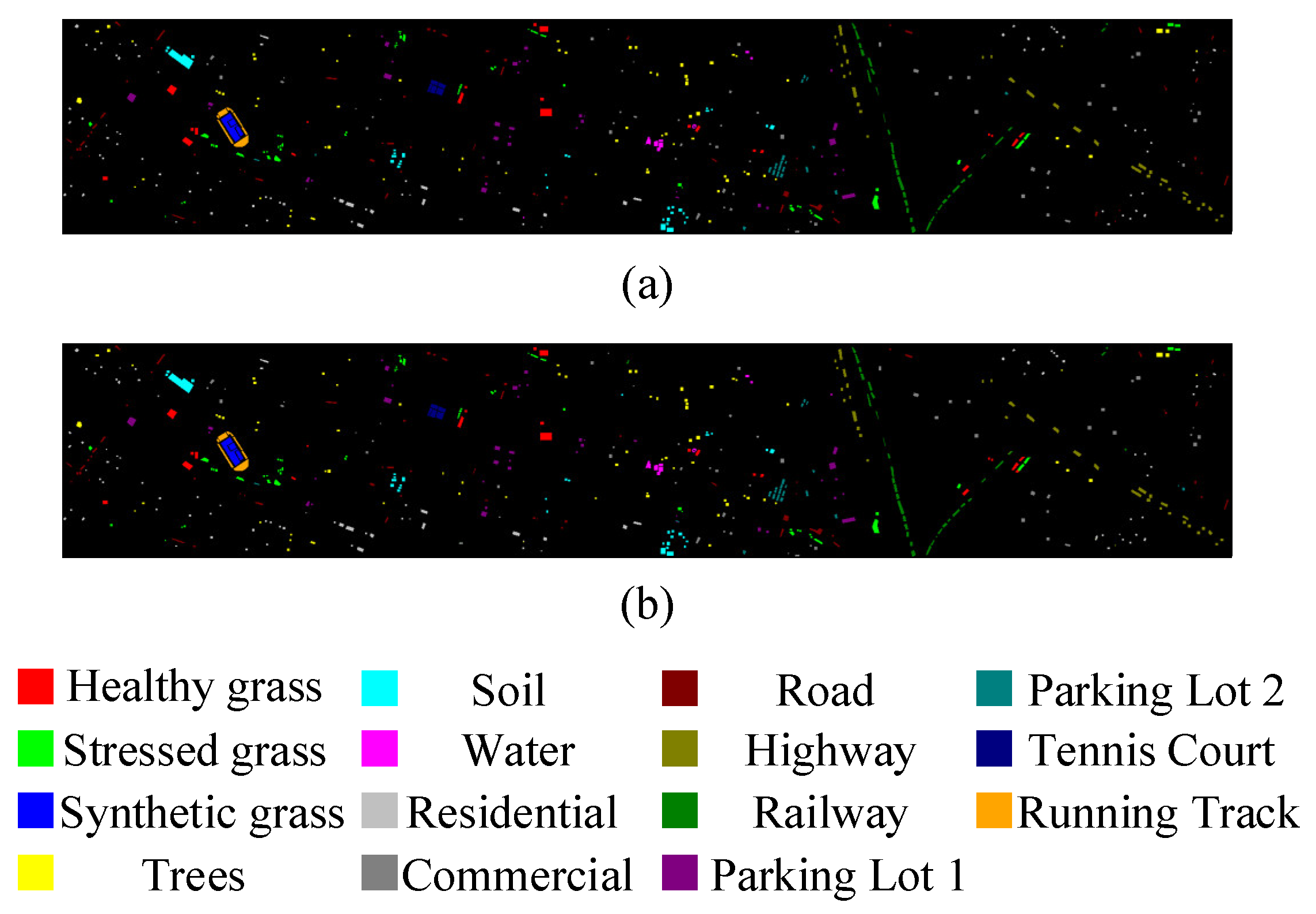
Figure 9.
Classification visualization results for HT datasets: (a) ground-truth map, and (b) map of the proposed method.
Figure 9.
Classification visualization results for HT datasets: (a) ground-truth map, and (b) map of the proposed method.

Figure 10.
Comparison of classification results using different attention mechanisms in the proposed method: (a) SE, (b) CBAM, and (c) 3DCAM.
Figure 10.
Comparison of classification results using different attention mechanisms in the proposed method: (a) SE, (b) CBAM, and (c) 3DCAM.

Figure 11.
Relationship between the training proportion and OA with different patch sizes of for the proposed 3DCAMNet: (a) IP dataset, (b) UP dataset, (c) KSC dataset, (d) SV dataset, and (e) HT dataset.
Figure 11.
Relationship between the training proportion and OA with different patch sizes of for the proposed 3DCAMNet: (a) IP dataset, (b) UP dataset, (c) KSC dataset, (d) SV dataset, and (e) HT dataset.

Figure 12.
Comparison of the OA values obtained by the method on the IP dataset.

Table 1.
Experimental dataset information.
| IP | UP | KSC | ||||||
|---|---|---|---|---|---|---|---|---|
| No. | Class | Number | No. | Class | Number | No. | Class | Number |
| 1 | Alfalfa | 46 | 1 | Asphalt | 6631 | 1 | Scrub | 761 |
| 2 | Corn-notill | 1428 | 2 | Meadows | 18,649 | 2 | Willow-swamp | 243 |
| 3 | Corn-mintill | 830 | 3 | Gravel | 2099 | 3 | CP-hammock | 256 |
| 4 | Corn | 237 | 4 | Trees | 3064 | 4 | Slash-pine | 252 |
| 5 | Grass/pasture | 483 | 5 | Painted metal sheets | 1345 | 5 | Oak/Broadleaf | 161 |
| 6 | Grass/trees | 730 | 6 | Bare Soil | 5029 | 6 | Hardwood | 229 |
| 7 | Grass/pasture-mowed | 28 | 7 | Bitumen | 1330 | 7 | Swap | 105 |
| 8 | Hay-windrowed | 478 | 8 | Self-Blocking Bricks | 3682 | 8 | Graminoid-marsh | 431 |
| 9 | Oats | 20 | 9 | Shadows | 947 | 9 | Spartina-marsh | 520 |
| 10 | Soybean-notill | 972 | / | / | / | 10 | Cattail-marsh | 404 |
| 11 | Soybean-mintill | 2455 | / | / | / | 11 | Salt-marsh | 419 |
| 12 | Soybean-clean | 593 | / | / | / | 12 | Mud-flats | 503 |
| 13 | Wheat | 205 | / | / | 13 | Water | 927 | |
| 14 | Woods | 1265 | / | / | / | / | / | / |
| 15 | Bldg-Grass-Tree-Drivers | 386 | / | / | / | / | / | / |
| 16 | Stone-Steel-Towers | 93 | / | / | / | / | / | / |
| Total | / | 10,249 | Total | / | 42,776 | Total | / | 5211 |
| SV | HT | |||||||
| No. | Class | Number | No. | Class | Number | |||
| 1 | Brocoil-green-weeds_1 | 2009 | 1 | Healthy grass | 1251 | |||
| 2 | Brocoil-green-weeds_2 | 3726 | 2 | Stressed grass | 1254 | |||
| 3 | Fallow | 1976 | 3 | Synthetic grass | 697 | |||
| 4 | Fallow-rough-plow | 1394 | 4 | Trees | 1244 | |||
| 5 | Fallow-smooth | 2678 | 5 | Soil | 1242 | |||
| 6 | Stubble | 3959 | 6 | Water | 325 | |||
| 7 | Celery | 3579 | 7 | Residential | 1268 | |||
| 8 | Grapes-untrained | 11,271 | 8 | Commercial | 1244 | |||
| 9 | Soil-vinyard-develop | 6203 | 9 | Road | 1252 | |||
| 10 | Corn-senesced-green-weeds | 3278 | 10 | Highway | 1227 | |||
| 11 | Lettuce-romaine-4wk | 1068 | 11 | Railway | 1235 | |||
| 12 | Lettuce-romaine-5wk | 1927 | 12 | Parking Lot 1 | 1233 | |||
| 13 | Lettuce-romaine-6wk | 916 | 13 | Parking Lot 2 | 469 | |||
| 14 | Lettuce-romaine-7wk | 1070 | 14 | Tennis Court | 428 | |||
| 15 | Vinyard-untrained | 7268 | 15 | Running Track | 660 | |||
| 16 | Vinyard-vertical-trellis | 1807 | / | / | / | |||
| Total | / | 54,129 | Total | / | 15,029 | |||
Table 2.
Superparameter setting of 3DCAMNet.
| Layer Name | Output Shape | Filter Size | Padding |
|---|---|---|---|
| Conv1 | 9 × 9 × L,24 | 1 × 1 × 7,24 | N |
| ConvBlock_1 | 9 × 9 × L,24 | 1 × 1 × 3,24 | Y |
| ConvBlock_2 | 9 × 9 × L,24 | 1 × 1 × 3,24 | Y |
| ConvBlock_3 | 9 × 9 × L,24 | 1 × 1 × 3,24 | Y |
| Avgpooling_h | 1 × 9 × 1,24 | / | / |
| Avgpooling_w | 9 × 1 × 1,24 | / | / |
| Avgpooling_l | 1 × 1 × L,24 | / | / |
| Conv_h | 1 × 9 × 1,24 | 1 × 1 × 1,24 | Y |
| Conv_w | 9 × 1 × 1,24 | 1 × 1 × 1,24 | Y |
| Conv_l | 1 × 1 × L,24 | 1 × 1 × 1,24 | Y |
| Linear Conv | 9 × 9 × L,48 | 1 × 1 × 1,48 | Y |
| Conv2 | 9 × 9 × 1,48 | 1 × 1 × L,48 | N |
| Avgpooling | 1 × 1 × 1,48 | / | / |
| Flatten(out) | class × 1 | 48 | N |
Table 3.
OA comparison of classification results obtained using different attention mechanisms (%).
| Datasets | SE | CBAM | 3DCAM |
|---|---|---|---|
| IP | 94.22 | 94.96 | 95.81 |
| UP | 96.92 | 96.64 | 97.01 |
| KSC | 98.32 | 98.51 | 99.01 |
| SV | 96.86 | 97.10 | 97.48 |
| HT | 97.30 | 97.43 | 97.69 |
Table 4.
OA value of different modules in 3DCAMNet (%).
| Modules | Linear Module | — | √ | — | √ |
|---|---|---|---|---|---|
| 3DCAM | — | — | √ | √ | |
| HSI datasets | IP | 95.02 | 95.78 | 95.00 | 95.81 |
| UP | 96.28 | 96.94 | 96.58 | 97.01 | |
| KSC | 98.33 | 98.80 | 98.75 | 99.01 | |
| SV | 96.20 | 96.56 | 96.87 | 97.48 | |
| HT | 96.28 | 97.14 | 97.25 | 97.69 |
Table 5.
Comparison of running time and parameters of different methods on IP dataset.
| Network | Input Size | Parameters | Running Time (s) |
|---|---|---|---|
| SSRN [52] | 9 × 9 × 200 | 364 k | 106 |
| PyResNet [40] | 9 × 9 × 200 | 22.4 M | 56 |
| DBMA [53] | 9 × 9 × 200 | 609 k | 222 |
| DBDA [55] | 9 × 9 × 200 | 382 k | 194 |
| Hybrid-SN [38] | 9 × 9 × 200 | 373 k | 37 |
| A2S2K-ResNet [57] | 9 × 9 × 200 | 403 k | 40 |
| 3DCAMNet | 9 × 9 × 200 | 423 k | 146 |
Publisher’s Note: MDPI stays neutral with regard to jurisdictional claims in published maps and institutional affiliations. |
© 2022 by the authors. Licensee MDPI, Basel, Switzerland. This article is an open access article distributed under the terms and conditions of the Creative Commons Attribution (CC BY) license (https://creativecommons.org/licenses/by/4.0/).
Share and Cite
MDPI and ACS Style
Shi, C.; Liao, D.; Zhang, T.; Wang, L. Hyperspectral Image Classification Based on 3D Coordination Attention Mechanism Network. Remote Sens. 2022, 14, 608. https://0-doi-org.brum.beds.ac.uk/10.3390/rs14030608
AMA Style
Shi C, Liao D, Zhang T, Wang L. Hyperspectral Image Classification Based on 3D Coordination Attention Mechanism Network. Remote Sensing. 2022; 14(3):608. https://0-doi-org.brum.beds.ac.uk/10.3390/rs14030608
Chicago/Turabian StyleShi, Cuiping, Diling Liao, Tianyu Zhang, and Liguo Wang. 2022. "Hyperspectral Image Classification Based on 3D Coordination Attention Mechanism Network" Remote Sensing 14, no. 3: 608. https://0-doi-org.brum.beds.ac.uk/10.3390/rs14030608
Note that from the first issue of 2016, this journal uses article numbers instead of page numbers. See further details here.