Article

Water Quality Retrieval from Landsat-9 (OLI-2) Imagery and Comparison to Sentinel-2

1
Digital Society Center, Fondazione Bruno Kessler, Via Sommarive 18, 38123 Trento, Italy
2
German Aerospace Center (DLR), Remote Sensing Technology Institute, Münchner Str. 20, Oberpfaffenhofen, D-82234 Weßling, Germany
3
Institute of Electromagnetic Sensing of the Environment, National Research Council of Italy (CNR-IREA), Via Corti 12, 20133 Milan, Italy
*
Author to whom correspondence should be addressed.
Remote Sens. 2022, 14(18), 4596; https://0-doi-org.brum.beds.ac.uk/10.3390/rs14184596
Submission received: 18 July 2022 / Revised: 30 August 2022 / Accepted: 13 September 2022 / Published: 14 September 2022
(This article belongs to the Special Issue Remote Sensing for Water Environment Monitoring)

Abstract

:
The Landsat series has marked the history of Earth observation by performing the longest continuous imaging program from space. The recent Landsat-9 carrying Operational Land Imager 2 (OLI-2) captures a higher dynamic range than sensors aboard Landsat-8 or Sentinel-2 (14-bit vs. 12-bit) that can potentially push forward the frontiers of aquatic remote sensing. This potential stems from the enhanced radiometric resolution of OLI-2, providing higher sensitivity over water bodies that are usually low-reflective. This study performs an initial assessment on retrieving water quality parameters from Landsat-9 imagery based on both physics-based and machine learning modeling. The concentration of chlorophyll-a (Chl-a) and total suspended matter (TSM) are retrieved based on physics-based inversion in four Italian lakes encompassing oligo to eutrophic conditions. A neural network-based regression model is also employed to derive Chl-a concentration in San Francisco Bay. We perform a consistency analysis between the constituents derived from Landsat-9 and near-simultaneous Sentinel-2 imagery. The Chl-a and TSM retrievals are validated using in situ matchups. The results indicate relatively high consistency among the water quality products derived from Landsat-9 and Sentinel-2. However, the Landsat-9 constituent maps show less grainy noise, and the matchup validation indicates relatively higher accuracies obtained from Landsat-9 (e.g., TSM R2 of 0.89) compared to Sentinel-2 (R2 = 0.71). The improved constituent retrieval from Landsat-9 can be attributed to the higher signal-to-noise (SNR) enabled by the wider dynamic range of OLI-2. We performed an image-based SNR estimation that confirms this assumption.

Graphical Abstract

1. Introduction

The launch of the first Landsat satellite dates back 50 years, which is followed by a series of satellites representing the longest continuous mission for Earth observation. Although the sensors aboard the Landsat series were not developed specifically for aquatic applications, water quality retrieval has been a key interest since the launch of the first Landsat satellites [1,2]. With the launch of Landsat-8 in 2013 carrying Operational Land Imager (OLI), remote sensing of biophysical parameters in optically-complex inland and near-shore coastal waters has become more widespread. Apart from other improvements of OLI compared to the previous Landsat sensors, its enhanced radiometric resolution (i.e., 12-bit dynamic range vs. 6-8 bit of previous sensors) paved the way to capture more subtle changes in water-leaving radiance [3,4]. The high radiometric resolution of satellite sensors is crucial for retrieving constituents, given that water bodies act as dark objects and absorb a major fraction of the downwelling irradiance leading to a low signal-to-noise ratio (SNR) [5]. With the launch of Sentinel-2 in 2015 carrying Multispectral Imager (MSI) that provides comparable characteristics with Landsat-8 (e.g., 12-bit dynamic range), remote sensing of inland waters has been further explored [6,7]. The newly launched Landsat-9 (in orbit since September 2021), with its onboard OLI-2 capturing 14-bit radiometric data, might resolve even smaller differences in water-leaving radiance relative to OLI and MSI that can potentially contribute to the studies on water quality retrieval. Satellite remote sensing provides an efficient means of retrieving spatially and temporally explicit information about the water quality indicators [8]. Remote mapping of chlorophyll-a (Chl-a) concentration, as an indicator of phytoplankton biomass, is of particular importance due to the ever-increasing eutrophication and algal bloom problems that pose a severe threat to inland and coastal waters [9,10]. Total suspended matter (TSM) mapping provides a measure of organic and mineral suspended solids, which is strongly related to water turbidity and might reveal information about mass transport and sediment re-suspension [11]. High loads of TSM can degrade primary production due to reduced light penetration in the water column and thus severely limits the aquatic habitat, fisheries, and drinking water supplies [12,13].
Various methods are developed for water quality retrieval from optical imagery, which are mainly empirical (regression-based) or physics-based models [14,15]. The empirical techniques require in situ measurements of constituents to form a relation between image-derived features (e.g., band ratios) and the water quality parameter of interest [16]. Various regressors can be employed for such empirically-based modeling, e.g., machine learning methods including neural networks and support vector machines [17,18]. Regression-based models are straightforward to apply as there is no need for a profound understanding of the underlying physics. However, these methods are mainly applicable when in situ samples concurrent with the image acquisition are available for training the regressor. Thus, in most cases, image-specific in situ data are needed as the transformation of the trained models is challenging either in space or time. Besides field measurements being timely and costly, they are very limited, if not available, particularly when analyzing imagery from a new satellite sensor. On the other hand, physics-based approaches invert a radiative transfer model that accounts for the absorption and backscattering properties of water and its optically active components, including Chl-a, TSM, and colored dissolved organic matter (CDOM) [19,20]. The inversion is mainly applied to the remote sensing reflectance (Rrs) derived after atmospheric correction [21,22]. There are mainly two approaches for physics-based inversion: (i) training a neural network using a large number of radiative transfer simulations and then using the trained model to estimate water quality parameters. As the constituent retrieval is based on pre-trained networks, there is no flexibility in adapting the retrieval to site-specific bio-optical conditions. Moreover, this approach is sensor-dependent and thus requires training an individual network for each sensor, such as those available in the Case 2 Regional CoastColour (C2RCC) processor [23]; (ii) analytical spectrum matching, which seeks an optimal match between the observed (image) spectrum and radiative transfer simulations by iterating a set of parameters in a given range, including the concentration of constituents. This inversion approach is sensor independent and highly flexible in parametrization. However, site-specific inherent optical properties (IOPs) such as the absorption spectrum of the phytoplankton are needed to optimize the inversion. Water Color Simulator (WASI) and Bio-Optical Model Based tool for Estimating water quality and bottom properties from Remote sensing images (BOMBER) are the main publically available processors based on the spectrum matching approach [22,24,25].
This study builds upon both physics-based and machine learning modeling to examine the water quality retrieval from newly released Landsat-9 imagery and compares the results with Sentinel-2. We examine the potential of OLI-2 data in retrieving Chl-a and TSM concentrations in the lake and near-shore coastal environments. We adapt the physics-based inversion implemented in BOMBER for the case studies with available site-specific IOPs (four Italian lakes). Moreover, a neural network (NN) empirical model is applied for a study site (San Francisco Bay) with a sufficient number of in situ data for training the model. In addition, we perform an inter-sensor comparison to quantify the consistency of Chl-a and TSM retrievals from Landsat-9 relative to Sentinel-2, a widely-used satellite sensor in water quality mapping, particularly in inland waters. Thus, we pursue the following objectives: (i) examine the potential of Landsat-9 imagery in retrieving Chl-a and TSM concentrations in lakes and near-shore coastal waters based on a fully physics-based approach as well as an empirical approach based on machine learning; (ii) perform a consistency analysis among the water quality products derived from Landsat-9 and Sentinel-2 and validate the results based on in situ matchups; (iii) compare the SNR from images acquired over different case studies as an indication for the radiometric quality of Landsat-9 data relative to Sentinel-2. Sensor noise is a limiting factor for detecting water constituents at low concentrations and resolving small concentration differences. Thus, this comparison indicates if sensor noise may explain some of the observed differences in the derived concentration maps.

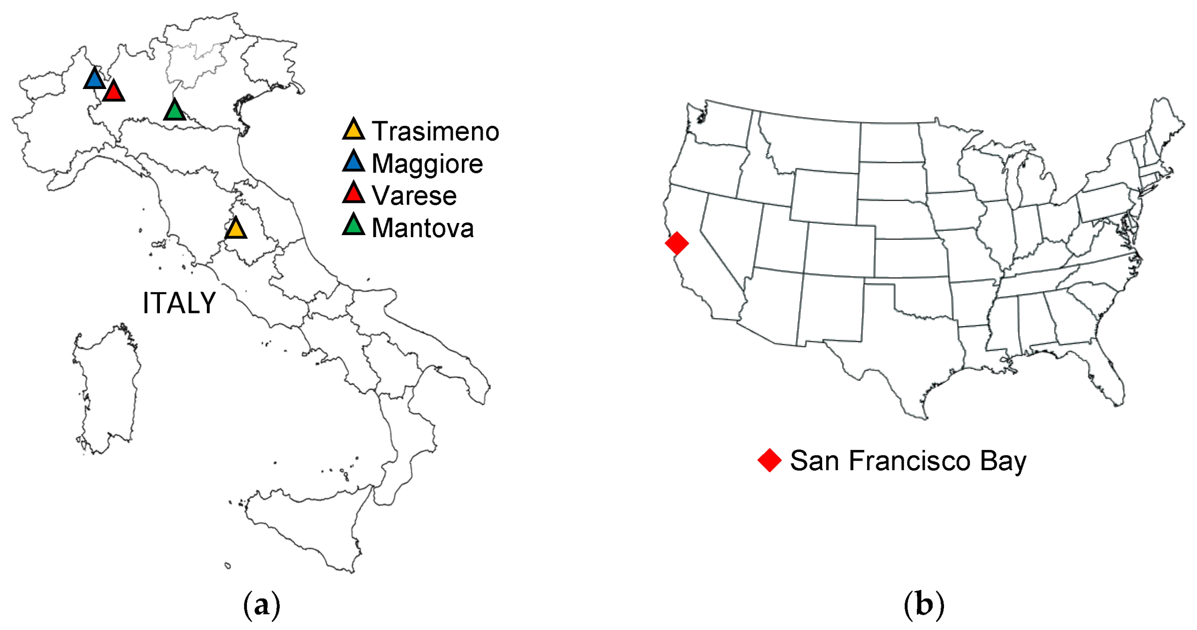
2. Case Studies and Datasets

Four Italian lakes named Trasimeno, Maggiore, Varese, and Mantova are considered for water quality retrieval from Landsat-9 and Sentinel-2 imagery (Figure 1a). The selected lakes represent a diverse bio-optical status (Table 1) involving oligo- to eutrophic conditions that allow for a relatively broad assessment of the constituent retrieval from satellite imagery. Moreover, the site-specific IOPs were available for these sites; thus, we consider them for physics-based inversion to retrieve Chl-a and TSM concentrations. We also investigated Chl-a retrieval in San Francisco Bay (Figure 1b), for which a sufficient number of in situ data (34 samples) was available to train an NN-based model. Samples of Landsat-9 and Sentinel-2 images, along with the location of in situ measurement stations, are shown in Figure 2 and Figure 3.
Table 1 reports the morphological characteristics and trophic status of case studies, along with the image acquisition dates. Moreover, the number of available in situ water quality matchups are provided for each water body during the studied period.
In situ data were collected by regional environmental protection agencies (i.e., ARPA Lombardia and ARPA Umbria) for Varese, Mantova, and Trasimeno lakes; integrated water samples between the surface and the Secchi Disk depth were collected using a Van Dorn water sampler. Chl-a concentrations extracted with acetone were determined via the spectrophotometric method [35]. TSM concentrations were determined gravimetrically [36]. Additional samples were collected with the WISPstation for Lake Trasimeno [37]. The water quality measurements of Lake Maggiore were provided by CNR-IRSA; the data are collected by fluorometer cyclops-7 installed on a fixed buoy [38]. The in situ Chl-a data at San Francisco Bay are based on fluorescence measurements calibrated with discrete Chl-a values according to U.S. Geological Survey (USGS) standards [34].
The relative spectral responses of Landsat-9 (OLI-2) and Sentinel-2 (MSI) are shown in Figure 4. The bands are presented for wavelengths λ < 1000 nm, which are the informative bands for retrieving water quality parameters. However, both sensors have three additional bands that are very similar, including one band at ~1370 nm for detection of clouds, particularly thin cirrus clouds, and two SWIR bands. Landsat-9 also provides a panchromatic band at 15 m spatial resolution. Moreover, carrying the thermal infrared sensor (TIR-2) allows the surface temperatures to be measured at 100 m spatial resolution. Instead, Sentinel-2 captures most of the useful bands for water quality retrieval at 10–20 m though the coastal blue band (443 nm) has a 60 m spatial resolution. Landsat-9 provides a revisit frequency of 16 days that enhances to eight days when coupled with Landsat-8. The constellation of Sentinel-2A and Sentinel-2B provides a temporal resolution of five days.
We downloaded level-1 top-of-atmosphere products of Landsat-9 and Sentinel-2. Then, dark spectrum fitting (DSF) atmospheric correction is performed using the ACOLITE processor [39,40] to derive Rrs data from both Landsat-9 and Sentinel-2 imagery. We use the same atmospheric correction for both sensors to maintain consistency in the analyses. To our knowledge, DSF is currently the only aquatic-specific atmospheric correction method available for processing the new Landsat-9 imagery. DSF has provided high-quality Rrs data in previous studies with various sensors, including Landsat-8 and Sentinel-2 [41,42,43]. The ancillary data (pressure, ozone, and water vapor) available through ACOLITE processor are used. However, a previous study demonstrated that the differences between using and not using ancillary data are very small [40]. Note that the Sentinel-2 images are resampled to 20 m through the ACOLITE atmospheric correction.

3. Methods

This study employs well-established physics-based and machine learning models to retrieve in-water constituents from Landsat-9 and Sentinel-2 imagery. Here, the methods are described briefly, and relevant references are provided for detailed information.

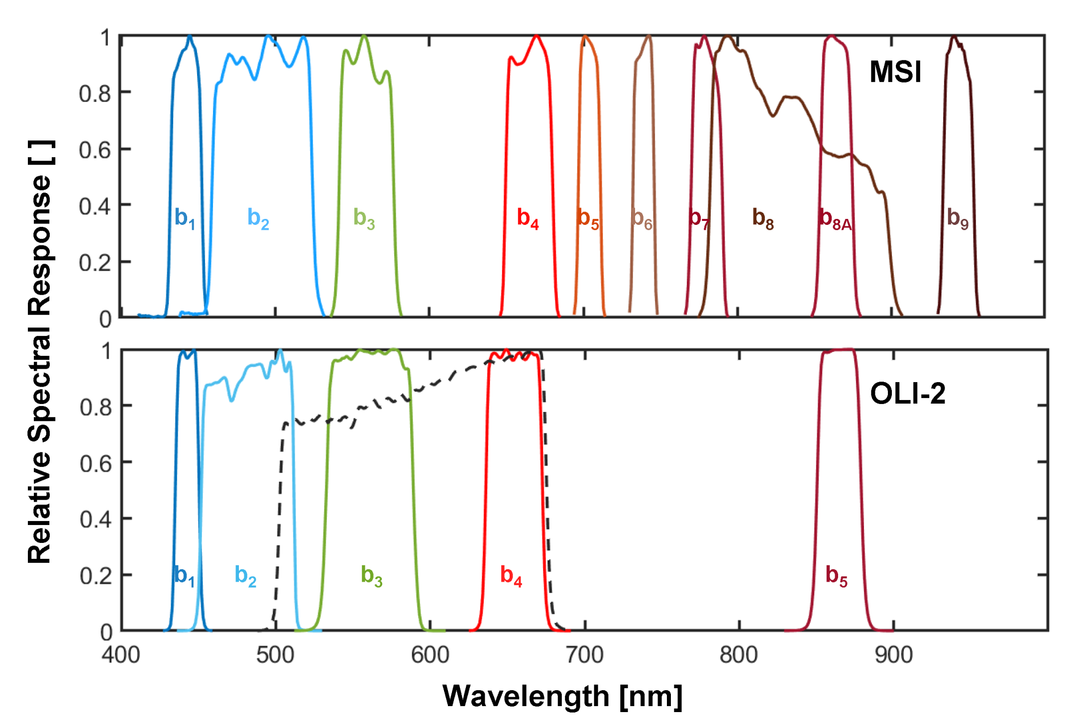
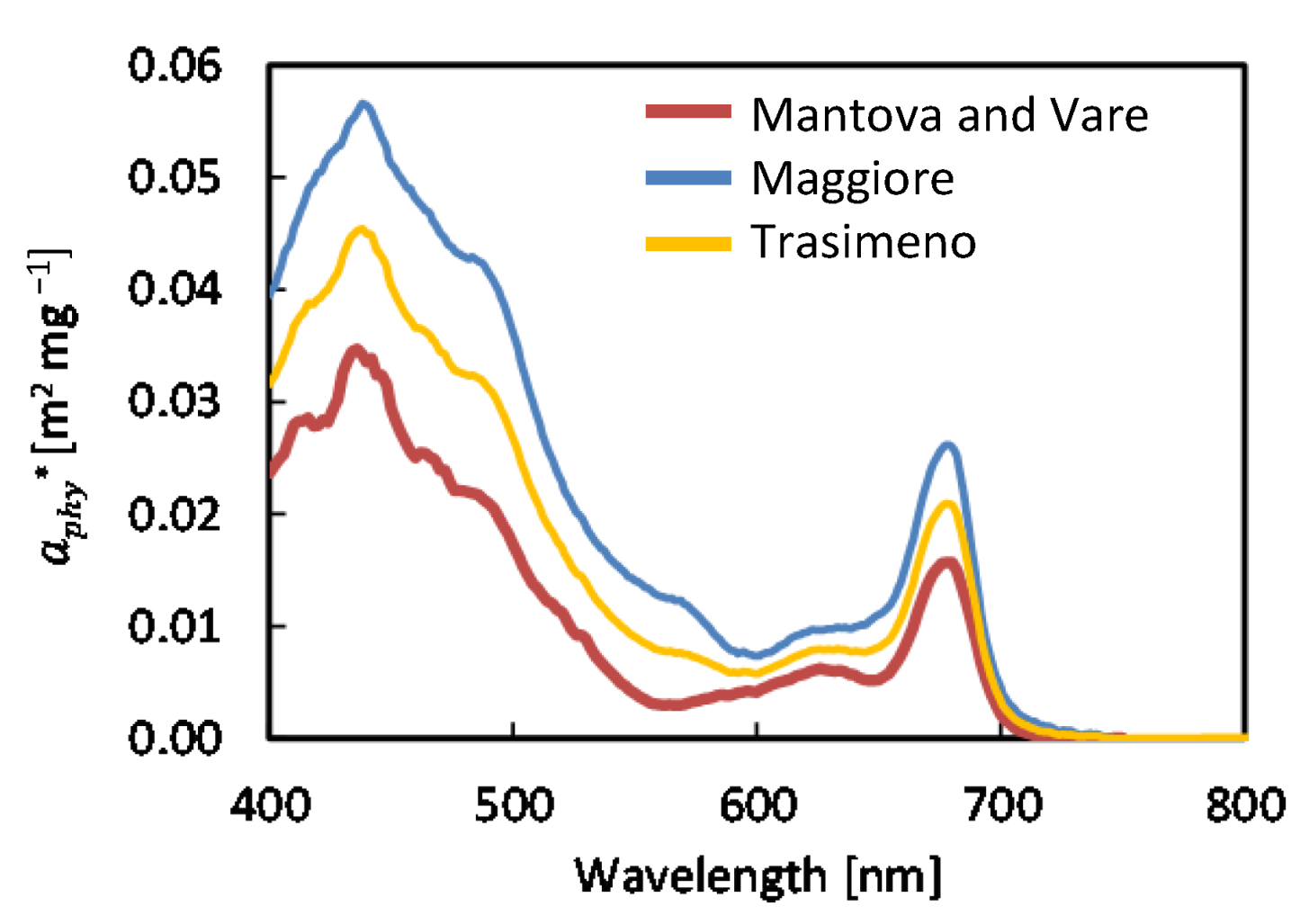
3.1. Physics-Based Model and Parametrization

We leverage BOMBER (Bio-Optical Model Based tool for Estimating water quality and bottom properties from Remote sensing images) as a physics-based inversion model to derive water quality parameters [24]. BOMBER is a publicly available processor (https://zenodo.org/record/5418571) that retrieves information about the water constituents and, in optically-shallow waters, bathymetry and substrate types/compositions. We apply BOMBER to Italian lakes (Section 2), for which the site-specific IOPs are available. For collecting the IOPs, the absorption spectra of particles retained on the filters were obtained using the filter pad technique, separately for phytoplankton and non-algal particles [36]. The spectrophotometric determination and processing were used to measure the absorption spectra of CDOM [44]. The backscattering coefficients of the particles were derived from HydroScat-6 measurements [45]. The lakes represent optically-deep conditions; thus, only water column properties are considered through the inversion process leading to the retrieval of TSM and Chl-a concentrations. The IOPs [26] of different lakes are reported in Table 2, which are used to parametrize BOMBER. Figure 5 shows the specific absorption spectra of phytoplankton a p h y * ( λ ) fed to the inversion model.

3.2. Neural Network-Based Regression Model

Empirical (regression-based) retrieval of constituents can be performed without knowing the site-specific IOPs and the underlying physics. However, in situ measurements of the parameters of interest are required to train the models. Polynomial regression models based on either single bands or band ratios have long been used for retrieving water quality parameters [7,46,47]. More recently, machine learning-based models, particularly neural networks (NNs), have received growing attention as they can handle the complex and non-linear relations between the spectral data and the target parameters (in water constituents). Here, we employ an NN-based regression model building upon feedforward fully connected layers similar to [18,48]. The network input data, i.e., spectral data of training samples, are connected to the first fully connected layer. Each fully connected layer performs a multiplication of input by a weight matrix and then adds a bias vector. The first fully connected layer is followed by an activation layer, and the last one produces the related water quality parameter (Figure 6). Bayesian optimization is applied to tune the network’s hyperparameters, including the number of layers, the number of neurons in each layer, and the type of the activation function. We apply the NN-based model to the imagery from San Francisco Bay, for which spatially-distributed Chl-a samples are available for training. Given the limited number of samples, we consider leave-one-out cross-validation to assess the Chl-a retrieval results. Thus, each sample is successively left out of the training data and used for validation [49].

3.3. Validation and Consistency Analysis

We employ several metrics, including coefficient of determination (R2), root mean square error/difference (RMSE/RMSD), bias, and mean absolute error (MAE), to perform in situ matchup validation and Landsat-9 vs. Sentinel-2 consistency analysis. Bias and MAE are both unitless and calculated in a log-transformed space to account for the proportionality of the errors with the water quality parameters according to the definition provided by [50]. Bias values tending to one are ideal, whereas bias > 1 indicates overestimation, and bias < 1 is an indication of underestimation. MAE is a multiplicative metric that always exceeds one and quantifies the relative error of water quality estimates. For instance, a MAE of 1.4 indicates a relative measurement error of 40%. In the case of error-free estimation, the MAE equals one. To relatively compare the RMSE/RMSD values among different case studies, we normalize them (NRMSE/NRMSD) with the average values of constituents. Note that, for the consistency analysis, water quality maps derived from Sentinel-2 at 20 m resolution are downsampled to 30 m to perform a pixel-by-pixel comparison with the maps derived from Landsat-9. We assume Sentinel-2 maps as the reference. Thus, for instance, a bias of 1.2 indicates that Landsat-9 retrievals are, on average, 20% higher than Sentinel-2.

3.4. Image-Based SNR Estimation

We employ a well-established approach for the estimation of SNR from satellite imagery. The local means and standard deviations of small homogeneous areas on a given image are calculated as an indication of the signal and noise, respectively [51]. Thus, the SNR of every band in a given image window is calculated by dividing the average of Rrs values by their standard deviation. We selected ten homogenous 5 × 5 windows for every case study and computed the average SNR.

4. Results and Discussion

Figure 7 illustrates the average Rrs spectra of different case studies derived from the DSF atmospheric correction using Landsat-9 and Sentinel-2 imagery. The spectra represent the average Rrs of each water body, excluding the boundary pixels. An additional Rrs spectrum is shown for the Varese Lake, representing a spot of the lake surface affected by a cyanobacterial bloom (see Figure 2: the greenish pattern crossing the middle of the lake).

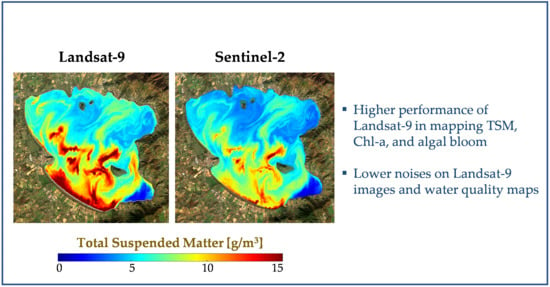
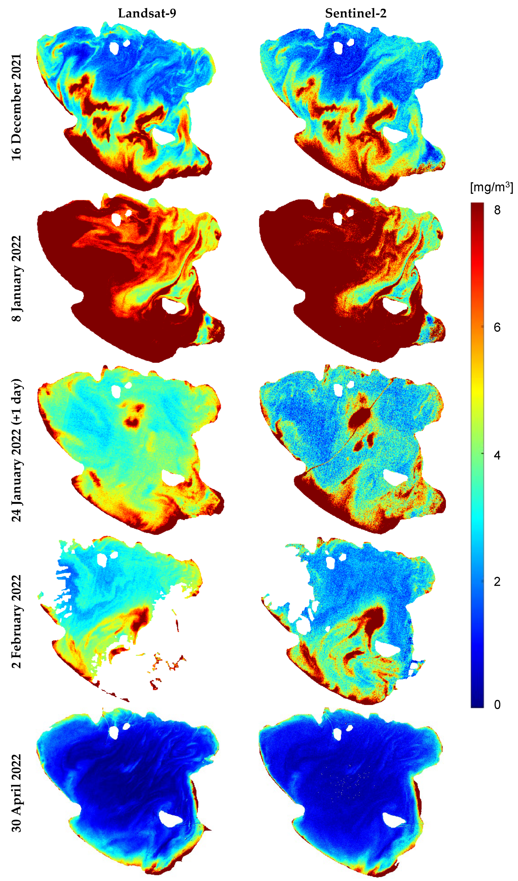
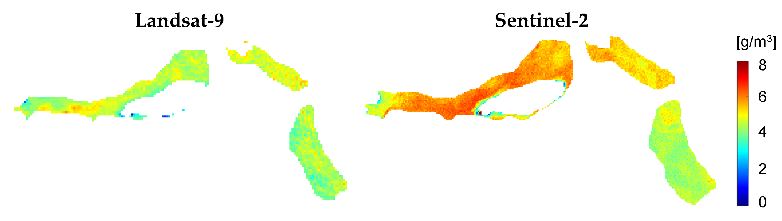
4.1. Physics-Based Inversion in Italian lakes

The TSM and Chl-a maps derived from multitemporal Landsat-9 and Sentinel-2 imagery of Lake Trasimeno are presented in Figure 8 and Figure 9. The visual inspection conveys a high correspondence between the Landsat-9 and Sentinel-2 retrievals though some differences are evident. Overall, the maps derived from Landsat-9 images, particularly Chl-a retrievals, are more homogenous and represent lower salt-and-pepper noises than those of Sentinel-2. The temporal analyses reveal that the concentration and pattern of constituents change significantly over time. The average TSM concentration ranges from ~5.8 g/m3 (2 February 2022) to ~16.1 g/m3 (8 January 2022). Similarly, a range of 3.8 mg/m3 to 10.5 mg/m3 is detected for Chl-a concentration. Note that the southeast corner of the lake is affected by the presence of macrophytes, and the water quality parameter estimation could be affected by the presence of shallow water. We have excluded this region from all analyses.
Figure 10 compares the Landsat-9 derived maps of TSM and Chl-a with those of Sentinel-2 in Lake Maggiore. Despite generic agreement in the spatial pattern of constituents, Sentinel-2 retrievals of TSM and Chl-a are lower than Landsat-9. The TSM maps derived from Landsat-9 and Sentinel-2 images of Lake Mantova are shown in Figure 11. Chl-a maps are not shown due to the noise caused by the poor signal in low light conditions and due to the dominant effect of TSM that prevails the upwelling radiance in this case study. Figure 12 shows the Chl-a maps retrieved from Landsat-9 and Sentinel-2 imagery in Lake Varese. As evident in the satellite images (Figure 2), there is a very contrasting pattern crossing from northwest to northeast of the lake. For the region dominated by this pattern (cyanobacterial bloom), the physics-based inversion infers a very high concentration of Chl-a from both Landsat-9 and Sentinel-2 imagery. TSM retrieval was not feasible due to the surface accumulation of cyanobacteria. This is because the signal recorded by the sensor is dominated by the surface component of radiance, and the contribution of the water column becomes negligible. In the lack of information from the water column, TSM retrieval would not be feasible regardless of the methods applied.
Example scatterplots analyzing the pixel-by-pixel TSM and Chl-a consistency between Landsat-9 and Sentinel-2 retrievals are shown in Figure 13 for Lake Trasimeno (16 December 2021). The consistency statistics for all multitemporal imagery of Lake Trasimeno and other case studies are reported in Table 3. For Lake Trasimeno, TSM maps show stronger agreement than Chl-a (average TSM R2 of 0.89 vs. 0.74 for Chl-a excluding 24 January data that the images have one day gap). However, Chl-a retrievals are slightly less biased (on average ~10%) than TSM when comparing Landsat-9 to Sentinel-2. In other lakes, the agreements of retrievals are not strong with relatively low R2 values. In Lake Maggiore, the bias values reported in Table 3 indicate that TSM and Chl-a values are, on average, 23% and 17% lower on Sentinel-2 maps compared to Landsat-9. In Lake Mantova, the Sentinel-2 map shows higher TSM (14% on average) with respect to Landsat-9. Despite the generic correspondence of the spatial patterns of maps derived from the two sensors in Lake Varese (Figure 12), the Sentinel-2-based retrievals of Chl-a are higher (60% on average) than those of Landsat-9 (Table 3). The NRMSD values are comparable in different case studies, particularly for TSM.
The in situ matchup analyses for TSM and Chl-a retrievals from Landsat-9 and Sentinel-2 imagery are presented in Table 4 for the studied lakes. Landsat-9 retrievals are more accurate than Sentinel-2 for both TSM and Chl-a, i.e., 0.18 improvement in R2 for TSM and 11.65 mg/m3 lower RMSE for Chl-a. As the Chl-a matchup analysis is strongly affected by the high concentration in Lake Varese, we performed an additional analysis excluding this sample that again confirms the outperformance of retrievals based on Landsat-9 imagery (R2 = 0.89 and RMSE = 0.75 mg/m3 for Landsat-9; R2 = 0.66 and RMSE = 1.86 mg/m3 for Sentinel-2).

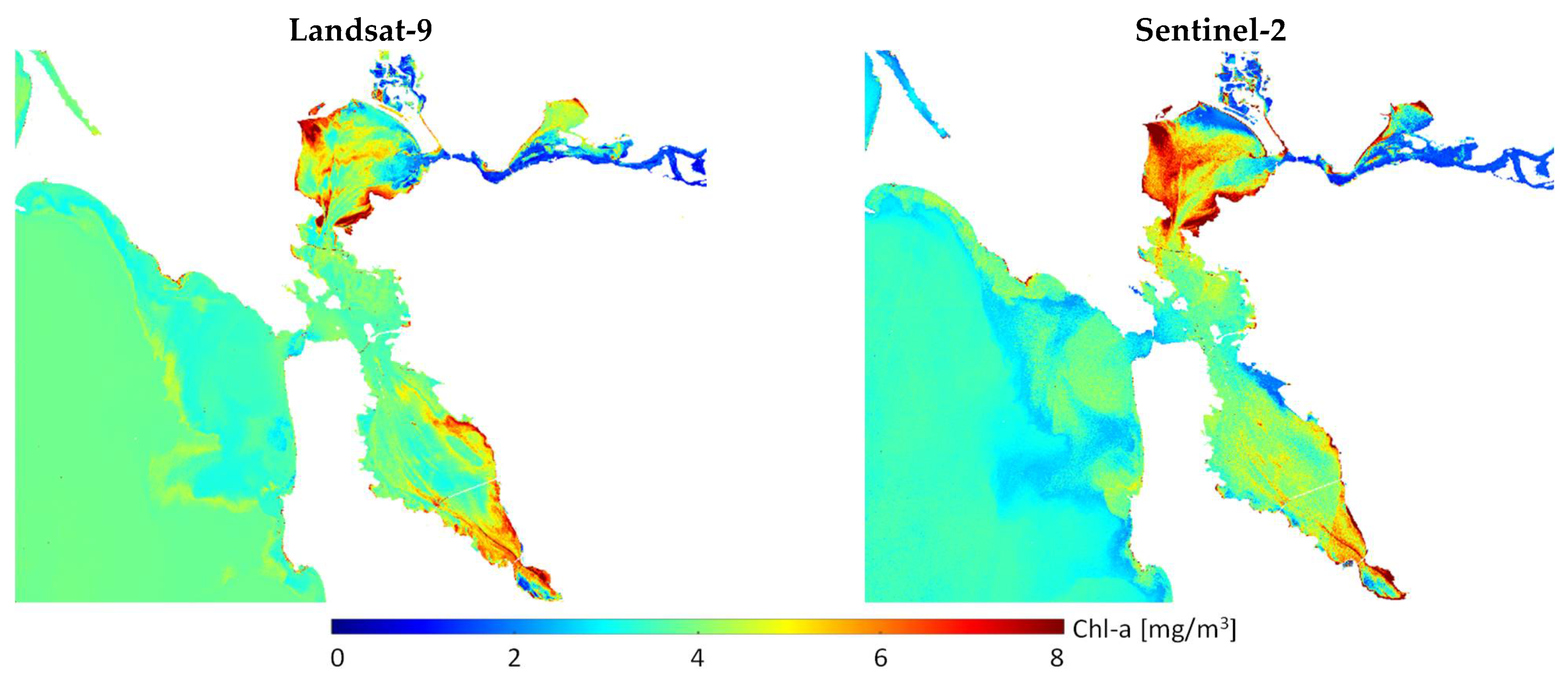
4.2. NN-Based Chl-a Retrieval in San Francisco Bay

The Chl-a maps of San Francisco Bay derived from Landsat-9 and Sentinel-2 images based on the NN regression model are presented in Figure 14. The pixel-by-pixel comparison implies a strong agreement between maps derived from Landsat-9 and Sentinel-2: R2 = 0.94, RMSD = 0.83 mg/m3, NRMSD = 16%, bias = 0.97, MAE = 1.13.
The in situ matchup validation is illustrated in Figure 15. The accuracies of Chl-a retrievals from Landsat-9 and Sentinel-2 are comparable though the former is slightly more accurate (Landsat-9 R2 of 0.85 vs. 0.8 for Sentinel-2).

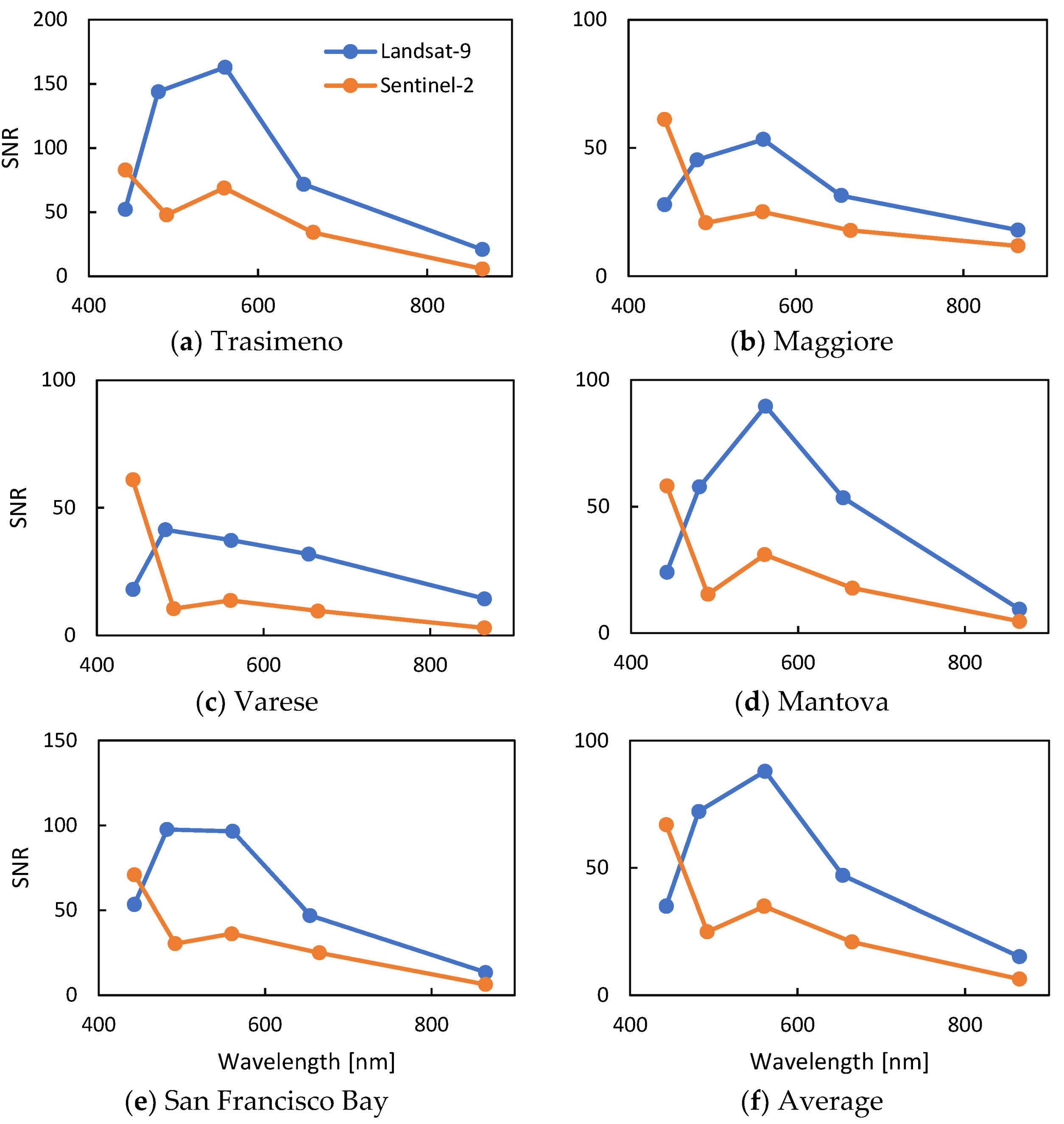
4.3. Image-Based SNR Estimation

The image-based SNR estimations (Section 3.4) over five similar bands of Landsat-9 and Sentinel-2 are shown in Figure 16. All case studies imply significantly higher SNR of Landsat-9 images relative to Sentinel-2 over all spectral channels except the coastal-blue band (443 nm). Although the magnitude of SNR depends on the case study, there are strong correspondences in the SNR trend over the spectrum for both sensors. Figure 16f illustrates the SNR averaged for all the case studies. The average SNR of Landsat-9 is higher than Sentinel-2 by a factor of 2.25 (red band) to 2.9 (blue band). However, the coastal-blue band of Sentinel-2 represents two times higher SNR than that of Landsat-9 on average.
Because sensor noise determines the thresholds for the absolute and relative concentrations of water constituents, concentration maps show a characteristic salt and pepper pattern close to these thresholds. Such a pattern is obvious in all Chl-a maps from lake Trasimeno (Figure 9) and the TSM map from 24 January 2022 (Figure 8) from Sentinel-2, while the Landsat-9 maps appear noise-free. This demonstrates that Landsat-9 has lower detection limits than Sentinel-2, particularly for Chl-a.

5. Conclusions

The recently launched Landsat-9 appeals to the aquatic remote sensing community as its onboard OLI-2 captures 16,384 brightness levels (14-bit data), notably higher than 4096 levels for Sentinel-2 (12-bit data). This enhanced radiometric resolution can provide more sensitivity to the water-leaving radiance than previous missions such as Landsat-8 and Sentinel-2 (12-bit dynamic range). This study examined the potential of Landsat-9 imagery in mapping lake and coastal water quality parameters. Landsat-9 provided improved retrievals of Chl-a and TSM compared to Sentinel-2 based on either the physics-based inversion or the NN regression model. This finding is consistent with a recent study on the bathymetric application of Landsat-9 imagery, demonstrating improved depth retrieval in fluvial systems compared to Sentinel-2 imagery [52]. The image-based SNR analysis supports the improved water quality results from Landsat-9. The Landsat-9 SNRs for four out of five common bands are remarkably (up to ~ three times) higher than Sentinel-2, which contributes to the accurate retrieval of constituents.
Although our analyses span several case studies, more investigation is needed to consider different water types and perform comprehensive validation with more in situ data. Our study compared the water quality products derived from Landsat-9 and Sentinel-2 imagery that indirectly provides insights into the quality of Rrs data that are the input for the inversion models. However, the assessment of Rrs products based on in situ reflectance measurements remains an area of investigation for future studies. The atmospheric correction methods also need further development and assessment for Landsat-9 imagery.

Author Contributions

Conceptualization, M.N.-J., F.B., M.B., P.G. and C.G.; methodology, M.N.-J., F.B., M.B., P.G. and C.G..; software, M.N.-J., M.B. and C.G.; validation, M.N.-J., M.B. and C.G.; formal analysis, M.N.-J., M.B. and C.G.; investigation, M.N.-J., M.B., P.G. and C.G.; resources, M.N.-J., F.B., M.B., P.G. and C.G.; data curation, M.N.-J., M.B., and C.G.; writing—original draft preparation, M.N.-J.; writing—review and editing, M.N.-J., F.B., M.B., P.G. and C.G.; visualization, M.N.-J. All authors have read and agreed to the published version of the manuscript.

Funding

This research received no external funding.

Data Availability Statement

The Landsat-9 and Sentinel-2 images are freely available at https://scihub.copernicus.eu/ and https://earthexplorer.usgs.gov/, respectively.

Acknowledgments

Authors would like to appreciate the in situ data provided by ARPA Lombardia and ARPA Umbria and the data provided by Andrea Lami from CNR-IRSA for Lake Maggiore. The Chl-a data from San Francisco Bay are provided by a USGS research program available at: https://sfbay.wr.usgs.gov/water-quality-database/ (accessed on 6 July 2022). M.B. and C.G. have conducted this study in the research framework of the H2020 Water-ForCE project (grant agreement No 101004186).

Conflicts of Interest

The authors declare no conflict of interest.

References

  1. Carpenter, D.J.; Carpenter, S.M. Modeling inland water quality using Landsat data. Remote Sens. Environ. 1983, 13, 345–352. [Google Scholar] [CrossRef]
  2. Munday, J.C.; Alföldi, T.T. LANDSAT test of diffuse reflectance models for aquatic suspended solids measurement. Remote Sens. Environ. 1979, 8, 169–183. [Google Scholar] [CrossRef]
  3. Gerace, A.D.; Schott, J.R.; Nevins, R. Increased potential to monitor water quality in the near-shore environment with Landsat’s next-generation satellite. J. Appl. Remote Sens. 2013, 7, 1–19. [Google Scholar] [CrossRef]
  4. Markogianni, V.; Kalivas, D.; Petropoulos, G.; Dimitriou, E. An Appraisal of the Potential of Landsat 8 in Estimating Chlorophyll-a, Ammonium Concentrations and Other Water Quality Indicators. Remote Sens. 2018, 10, 1018. [Google Scholar] [CrossRef]
  5. Jorge, D.S.F.; Barbosa, C.C.F.; De Carvalho, L.A.S.; Affonso, A.G.; Lobo, F.D.L.; Novo, E.M.L.D.M. SNR (Signal-To-Noise Ratio) Impact on Water Constituent Retrieval from Simulated Images of Optically Complex Amazon Lakes. Remote Sens. 2017, 9, 644. [Google Scholar] [CrossRef]
  6. Sent, G.; Biguino, B.; Favareto, L.; Cruz, J.; Sá, C.; Dogliotti, A.I.; Palma, C.; Brotas, V.; Brito, A.C. Deriving Water Quality Parameters Using Sentinel-2 Imagery: A Case Study in the Sado Estuary, Portugal. Remote Sens. 2021, 13, 1043. [Google Scholar] [CrossRef]
  7. Toming, K.; Kutser, T.; Laas, A.; Sepp, M.; Paavel, B.; Nõges, T. First Experiences in Mapping Lake Water Quality Parameters with Sentinel-2 MSI Imagery. Remote Sens. 2016, 8, 640. [Google Scholar] [CrossRef]
  8. Ritchie, J.C.; Zimba, P.V.; Everitt, J.H. Remote Sensing Techniques to Assess Water Quality. Photogramm. Eng. Remote Sens. 2003, 69, 695–704. [Google Scholar] [CrossRef]
  9. Caballero, I.; Fernández, R.; Escalante, O.M.; Mamán, L.; Navarro, G. New capabilities of Sentinel-2A/B satellites combined with in situ data for monitoring small harmful algal blooms in complex coastal waters. Sci. Rep. 2020, 10, 8743. [Google Scholar] [CrossRef]
  10. Binding, C.E.; Greenberg, T.A.; McCullough, G.; Watson, S.B.; Page, E. An analysis of satellite-derived chlorophyll and algal bloom indices on Lake Winnipeg. J. Great Lakes Res. 2018, 44, 436–446. [Google Scholar] [CrossRef]
  11. Rodrigues, T.; Mishra, D.R.; Alcantara, E.; Watanabe, F.; Rotta, L.; Imai, N.N. Retrieving Total Suspended Matter in Tropical Reservoirs Within a Cascade System with Widely Differing Optical Properties. IEEE J. Sel. Top. Appl. Earth Obs. Remote Sens. 2017, 10, 5495–5512. [Google Scholar] [CrossRef]
  12. Soomets, T.; Uudeberg, K.; Jakovels, D.; Brauns, A.; Zagars, M.; Kutser, T. Validation and comparison of water quality products in baltic lakes using sentinel-2 msi and sentinel-3 OLCI data. Sensors 2020, 20, 742. [Google Scholar] [CrossRef]
  13. Giardino, C.; Bresciani, M.; Braga, F.; Cazzaniga, I.; De Keukelaere, L.; Knaeps, E.; Brando, V.E. Chapter 5—Bio-optical Modeling of Total Suspended Solids. In Bio-Optical Modeling and Remote Sensing of Inland Water; Mishra, D.R., Ogashawara, I., Gitelson, A.A., Eds.; Elsevier: Amsterdam, The Netherlands, 2017; pp. 129–156. ISBN 978-0-12-804644-9. [Google Scholar]
  14. Odermatt, D.; Gitelson, A.; Brando, V.E.; Schaepman, M. Review of constituent retrieval in optically deep and complex waters from satellite imagery. Remote Sens. Environ. 2012, 118, 116–126. [Google Scholar] [CrossRef]
  15. Niroumand-Jadidi, M.; Bovolo, F.; Bruzzone, L.; Gege, P. Inter-Comparison of Methods for Chlorophyll-a Retrieval: Sentinel-2 Time-Series Analysis in Italian Lakes. Remote Sens. 2021, 13, 2381. [Google Scholar] [CrossRef]
  16. Niroumand-Jadidi, M.; Bovolo, F.; Bruzzone, L. Novel Spectra-Derived Features for Empirical Retrieval of Water Quality Parameters: Demonstrations for OLI, MSI, and OLCI Sensors. IEEE Trans. Geosci. Remote Sens. 2019, 57, 10285–10300. [Google Scholar] [CrossRef]
  17. Hafeez, S.; Wong, M.S.; Ho, H.C.; Nazeer, M.; Nichol, J.; Abbas, S.; Tang, D.; Lee, K.H.; Pun, L. Comparison of Machine Learning Algorithms for Retrieval of Water Quality Indicators in Case-II Waters: A Case Study of Hong Kong. Remote Sens. 2019, 11, 617. [Google Scholar] [CrossRef]
  18. Niroumand-Jadidi, M.; Bovolo, F. Temporally Transferable Machine Learning Model for Total Suspended Matter Retrieval from Sentinel-2. ISPRS Ann. Photogramm. Remote Sens. Spat. Inf. Sci. 2022, 3, 339–345. [Google Scholar] [CrossRef]
  19. Niroumand-Jadidi, M.; Bovolo, F.; Bruzzone, L.; Gege, P. Physics-based Bathymetry and Water Quality Retrieval Using PlanetScope Imagery: Impacts of 2020 COVID-19 Lockdown and 2019 Extreme Flood in the Venice Lagoon. Remote Sens. 2020, 12, 2381. [Google Scholar] [CrossRef]
  20. Niroumand-Jadidi, M.; Bovolo, F.; Bruzzone, L. Water Quality Retrieval from PRISMA Hyperspectral Images: First Experience in a Turbid Lake and Comparison with Sentinel-2. Remote Sens. 2020, 12, 3984. [Google Scholar] [CrossRef]
  21. Mobley, C.D. Light and Water: Radiative Transfer in Natural Waters; Academic Press: Cambridge, MA, USA, 1994; ISBN 9780125027502. [Google Scholar]
  22. Gege, P. The water color simulator WASI: An integrating software tool for analysis and simulation of optical in situ spectra. Comput. Geosci. 2004, 30, 523–532. [Google Scholar] [CrossRef]
  23. Brockmann, C.; Doerffer, R.; Peters, M.; Stelzer, K.; Embacher, S.; Ruescas, A. Evolution of the C2RCC neural network for Sentinel 2 and 3 for the retrieval of ocean colour products in normal and extreme optically complex waters. In Proceedings of the ESA Living Planet, Prague, Czech Republic, 9–13 May 2016. [Google Scholar]
  24. Giardino, C.; Candiani, G.; Bresciani, M.; Lee, Z.; Gagliano, S.; Pepe, M. BOMBER: A tool for estimating water quality and bottom properties from remote sensing images. Comput. Geosci. 2012, 45, 313–318. [Google Scholar] [CrossRef]
  25. Gege, P. WASI-2D: A software tool for regionally optimized analysis of imaging spectrometer data from deep and shallow waters. Comput. Geosci. 2014, 62, 208–215. [Google Scholar] [CrossRef]
  26. Bresciani, M.; Giardino, C.; Fabbretto, A.; Pellegrino, A.; Mangano, S.; Free, G.; Pinardi, M. Application of New Hyperspectral Sensors in the Remote Sensing of Aquatic Ecosystem Health: Exploiting PRISMA and DESIS for Four Italian Lakes. Resources 2022, 11, 8. [Google Scholar] [CrossRef]
  27. Free, G.; Bresciani, M.; Pinardi, M.; Peters, S.; Laanen, M.; Padula, R.; Cingolani, A.; Charavgis, F.; Giardino, C. Shorter blooms expected with longer warm periods under climate change: An example from a shallow meso-eutrophic Mediterranean lake. Hydrobiologia 2022. [Google Scholar] [CrossRef]
  28. Eleveld, M.A.; Ruescas, A.B.; Hommersom, A.; Moore, T.S.; Peters, S.W.M.; Brockmann, C. An Optical Classification Tool for Global Lake Waters. Remote Sens. 2017, 9, 420. [Google Scholar] [CrossRef]
  29. Giardino, C.; Bresciani, M.; Stroppiana, D.; Oggioni, A.; Morabito, G. Optical remote sensing of lakes: An overview on Lake Maggiore. J. Limnol. 2013, 73, 817. [Google Scholar] [CrossRef]
  30. Chirico, N.; António, D.C.; Pozzoli, L.; Marinov, D.; Malagó, A.; Sanseverino, I.; Beghi, A.; Genoni, P.; Dobricic, S.; Lettieri, T. Cyanobacterial Blooms in Lake Varese: Analysis and Characterization over Ten Years of Observations. Water 2020, 12, 675. [Google Scholar] [CrossRef]
  31. Bresciani, M.; Giardino, C.; Lauceri, R.; Matta, E.; Cazzaniga, I.; Pinardi, M.; Lami, A.; Austoni, M.; Viaggiu, E.; Congestri, R.; et al. Earth observation for monitoring and mapping of cyanobacteria blooms. Case studies on five Italian lakes. J. Limnol. 2016, 76, 1565. [Google Scholar] [CrossRef]
  32. Pinardi, M.; Bresciani, M.; Villa, P.; Cazzaniga, I.; Laini, A.; Tóth, V.; Fadel, A.; Austoni, M.; Lami, A.; Giardino, C. Spatial and temporal dynamics of primary producers in shallow lakes as seen from space: Intra-annual observations from Sentinel-2A. Limnologica 2018, 72, 32–43. [Google Scholar] [CrossRef]
  33. Taylor, N.C.; Kudela, R.M. Spatial Variability of Suspended Sediments in San Francisco Bay, California. Remote Sens. 2021, 13, 4625. [Google Scholar] [CrossRef]
  34. Schraga, T.S.; Cloern, J.E. Water quality measurements in San Francisco Bay by the U.S. Geological Survey, 1969–2015. Sci. Data 2017, 4, 170098. [Google Scholar] [CrossRef] [PubMed]
  35. APAT Metodi Analitici per le Acque. Available online: https://www.isprambiente.gov.it/it/pubblicazioni/manuali-e-linee-guida/metodi-analitici-per-le-acque (accessed on 4 November 2020).
  36. Strömbeck, N.; Pierson, D.C. The effects of variability in the inherent optical properties on estimations of chlorophyll a by remote sensing in Swedish freshwaters. Sci. Total Environ. 2001, 268, 123–137. [Google Scholar] [CrossRef]
  37. Bresciani, M.; Pinardi, M.; Free, G.; Luciani, G.; Ghebrehiwot, S.; Laanen, M.; Peters, S.; Della Bella, V.; Padula, R.; Giardino, C. The Use of Multisource Optical Sensors to Study Phytoplankton Spatio-Temporal Variation in a Shallow Turbid Lake. Water 2020, 12, 284. [Google Scholar] [CrossRef]
  38. Tiberti, R.; Caroni, R.; Cannata, M.; Lami, A.; Manca, D.; Strigaro, D.; Rogora, M. Automated high frequency monitoring of Lake Maggiore through in situ sensors: System design, field test and data quality control. J. Limnol. 2021, 80, 2011. [Google Scholar] [CrossRef]
  39. Vanhellemont, Q. Adaptation of the dark spectrum fitting atmospheric correction for aquatic applications of the Landsat and Sentinel-2 archives. Remote Sens. Environ. 2019, 225, 175–192. [Google Scholar] [CrossRef]
  40. Vanhellemont, Q. Sensitivity analysis of the dark spectrum fitting atmospheric correction for metre- and decametre-scale satellite imagery using autonomous hyperspectral radiometry. Opt. Express 2020, 28, 29948–29965. [Google Scholar] [CrossRef] [PubMed]
  41. Pereira-Sandoval, M.; Ruescas, A.; Urrego, P.; Ruiz-Verdú, A.; Delegido, J.; Tenjo, C.; Soria-Perpinyà, X.; Vicente, E.; Soria, J.; Moreno, J. Evaluation of Atmospheric Correction Algorithms over Spanish Inland Waters for Sentinel-2 Multi Spectral Imagery Data. Remote Sens. 2019, 11, 1469. [Google Scholar] [CrossRef]
  42. Vanhellemont, Q.; Ruddick, K. Atmospheric correction of Sentinel-3/OLCI data for mapping of suspended particulate matter and chlorophyll-a concentration in Belgian turbid coastal waters. Remote Sens. Environ. 2021, 256, 112284. [Google Scholar] [CrossRef]
  43. Caballero, I.; Román, A.; Tovar-Sánchez, A.; Navarro, G. Water quality monitoring with Sentinel-2 and Landsat-8 satellites during the 2021 volcanic eruption in La Palma (Canary Islands). Sci. Total Environ. 2022, 822, 153433. [Google Scholar] [CrossRef]
  44. Kirk, J.T.O. Light and Photosynthesis in Aquatic Ecosystems, 2nd ed.; Cambridge University Press: Cambridge, UK, 1994. [Google Scholar]
  45. Maffione, R.A.; Dana, D.R. Instruments and methods for measuring the backward-scattering coefficient of ocean waters. Appl. Opt. 1997, 36, 6057–6067. [Google Scholar] [CrossRef]
  46. Dekker, A.G.; Peters, S.W.M. The use of the Thematic Mapper for the analysis of eutrophic lakes: A case study in the Netherlands. Int. J. Remote Sens. 1993, 14, 799–821. [Google Scholar] [CrossRef]
  47. Han, L.; Jordan, K.J. Estimating and mapping chlorophyll- a concentration in Pensacola Bay, Florida using Landsat ETM+ data. Int. J. Remote Sens. 2005, 26, 5245–5254. [Google Scholar] [CrossRef]
  48. Niroumand-Jadidi, M.; Legleiter, C.J.; Bovolo, F. Bathymetry retrieval from CubeSat image sequences with short time lags. Int. J. Appl. Earth Obs. Geoinf. 2022, 112, 102958. [Google Scholar] [CrossRef]
  49. Arlot, S.; Celisse, A. A survey of cross-validation procedures for model selection. Stat. Surv. 2010, 4, 40–79. [Google Scholar] [CrossRef]
  50. Seegers, B.N.; Stumpf, R.P.; Schaeffer, B.A.; Loftin, K.A.; Werdell, P.J. Performance metrics for the assessment of satellite data products: An ocean color case study. Opt. Express 2018, 26, 7404. [Google Scholar] [CrossRef]
  51. Gao, B.-C. An operational method for estimating signal to noise ratios from data acquired with imaging spectrometers. Remote Sens. Environ. 1993, 43, 23–33. [Google Scholar] [CrossRef]
  52. Niroumand-Jadidi, M.; Legleiter, C.J.; Bovolo, F. River Bathymetry Retrieval From Landsat-9 Images Based on Neural Networks and Comparison to SuperDove and Sentinel-2. IEEE J. Sel. Top. Appl. Earth Obs. Remote Sens. 2022, 15, 5250–5260. [Google Scholar] [CrossRef]
Figure 1. The location of studied (a) lakes in Italy and (b) San Francisco Bay in the United States.
Remotesensing 14 04596 g001
Figure 2. True color composite Landsat-9 and near-simultaneous Sentinel-2 images over four Italian lakes. The locations of in situ stations are shown on Landsat-9 images by yellow symbols.
Remotesensing 14 04596 g002
Figure 3. True color composite Landsat-9 and near-simultaneous Sentinel-2 images over San Francisco Bay. The locations of in situ stations are shown on Landsat-9 images by yellow symbols.
Remotesensing 14 04596 g003
Figure 4. Relative spectral response of OLI-2 and MSI onboard Landsat-9 and Sentinel-2, respectively. The band numbers are provided for each sensor, and the gray dashed line shows Landsat-9 panchromatic band.
Remotesensing 14 04596 g004
Figure 5. The specific absorption spectrum of phytoplankton a p h y * ( λ ) in Italian lakes.
Remotesensing 14 04596 g005
Figure 6. Schematic representation of training NN model for Chl-a retrieval in San Francisco Bay.
Remotesensing 14 04596 g006
Figure 7. Remote sensing reflectance (Rrs) spectra derived from DSF atmospheric correction over different case studies using (a) Landsat-9 and (b) Sentinel-2 imagery.
Remotesensing 14 04596 g007
Figure 8. TSM maps derived from Landsat-9 and Sentinel-2 imagery in Lake Trasimeno using BOMBER.
Remotesensing 14 04596 g008
Figure 9. Chl-a maps derived from Landsat-9 and Sentinel-2 imagery in Lake Trasimeno using BOMBER.
Remotesensing 14 04596 g009
Figure 10. TSM and Chl-a maps derived from Landsat-9 and Sentinel-2 imagery in Lake Maggiore.
Remotesensing 14 04596 g010
Figure 11. TSM maps derived from Landsat-9 and Sentinel-2 imagery in Lake Mantova.
Remotesensing 14 04596 g011
Figure 12. Chl-a map derived from Landsat-9 and Sentinel-2 imagery in Lake Varese.
Remotesensing 14 04596 g012
Figure 13. Pixel-by-pixel comparison of (a) TSM and (b) Chl-a maps derived from Landsat-9 vs. Sentinel-2 in Lake Trasimeno (16 December 2021).
Remotesensing 14 04596 g013
Figure 14. Chl-a maps derived from Landsat-9 and Sentinel-2 imagery in San Francisco Bay based on NN regression model.
Remotesensing 14 04596 g014
Figure 15. In situ matchup validation of Chl-a retrieval from Landsat-9 and Sentinel-2 imagery in San Francisco Bay.
Remotesensing 14 04596 g015
Figure 16. Image-based SNR estimates of Landsat-9 and Sentinel-2 for each case study.
Remotesensing 14 04596 g016
Table 1. Site descriptions, image acquisition dates, and the number of in situ samples for each case study.
Water BodySite DescriptionsLandsat-9 Imagery
(Sentinel-2 Overpass)
Number of In Situ Matchups
Trasimeno LakeSurface area: 120.5 km2
Shallow (max depth ~6.3 m), turbid (Secchi depth ~1.1 m), and mesotrophic–eutrophic lake [26,27]
16 December 2021 (same day)
8 January 2022 (same day)
24 January 2022 (+1 day)
2 February 2022 (same day)
30 April 2022 (same day)
4 Chl-a
2 TSM
Maggiore LakeSurface area ~212.5 km2, represents deep water up to 370 m, oligotrophic lake [28], Secchi depth ~10 m [29]29 January 2022 (same day)1 Chl-a
1 TSM
Varese LakeSurface area ~14.8 km2, mean depth ~11 m; Secchi depth ~3 m [30]. A dimictic lake with a summer stratification from May to November and an inverse stratification in winter [31]5 December 2021 (same day)1 Chl-a
Mantova LakeSurface area: 6.2 km2; mean depth ~3.5 m; a hypertrophic system composed of three fluvial lakes with low transparency (Secchi depth < 1 m in summer and high Chl-a concentration) [31,32] 9 February 2022 (−2 days)3 Chl-a
3 TSM
San Francisco BaySurface area: ~1400 km2; most extensive estuary system on the west coast of North America, overall a shallow water body (<3 m in most parts) but also representing deep waters up to ~113 m, turbid with an average TSM of ~30 g/m3 for the past year [33,34]10 December 2021 (same day)34 Chl-a
Table 2. Site-specific inherent optical properties (IOPs) of Italian lakes used for parametrizing BOMBER.
TrasimenoMaggioreVarese and Mantova
Spectral slope coefficient of CDOM absorption [1/nm]0.0160.0190.015
Specific absorption of non-algal particles (NAP) at 440 nm [m2/g]0.20.050.3
Spectral slope coefficient of NAP absorption [1/nm]0.0130.0110.009
Backscattering exponent of TSM [−]0.650.760.8
Specific backscattering coefficient of TSM at 555 nm [m2/g]0.01190.00710.0111
Table 3. Consistency analysis of TSM and Chl-a concentrations derived from Landsat-9 and Sentinel-2 via BOMBER in Italian lakes.
R2RMSDNRMSD%BiasMAE
Trasimeno
16 December 2021
TSM0.871.78 g/m3221.241.24
Chl-a0.770.94 mg/m3211.051.25
Trasimeno
8 January 2022
TSM0.904.56 g/m3200.921.18
Chl-a0.925.63 mg/m3380.791.36
Trasimeno
24 January 2022
TSM0.311.03 g/m3140.931.14
Chl-a0.301.19 mg/m3261.211.32
Trasimeno
2 February 2022
TSM0.821.50 g/m3251.401.41
Chl-a0.590.93 mg/m3241.271.31
Trasimeno
30 April 2022
TSM0.970.66 g/m390.901.10
Chl-a0.690.44 mg/m3280.881.54
MaggioreTSM0.330.16 g/m3201.231.24
Chl-a0.060.49 mg/m3191.171.18
MantovaTSM0.170.99 g/m3190.861.18
VareseChl-a0.1361.7 mg/m3550.402.52
Table 4. In situ matchup validation of TSM (6 samples) and Chl-a (9 samples) retrievals via BOMBER from Landsat-9 and Sentinel-2 imagery in the studied lakes.
R2RMSENRMSE%BiasMAE
TSMLandsat-90.890.77 g/m3181.011.17
Sentinel-20.711.20 g/m3271.041.27
Chl-aLandsat-90.991.05 mg/m351.031.16
Sentinel-20.9712.7 mg/m3551.011.27
Publisher’s Note: MDPI stays neutral with regard to jurisdictional claims in published maps and institutional affiliations.

