Article

Comparison of Ground Point Filtering Algorithms for High-Density Point Clouds Collected by Terrestrial LiDAR

1
Department of Geography & Sustainability, University of Tennessee, Knoxville, TN 37996, USA
2
Department of Biosystems Engineering & Soil Science, University of Tennessee, Knoxville, TN 37996, USA
*
Author to whom correspondence should be addressed.
Remote Sens. 2022, 14(19), 4776; https://0-doi-org.brum.beds.ac.uk/10.3390/rs14194776
Submission received: 3 August 2022 / Revised: 8 September 2022 / Accepted: 22 September 2022 / Published: 24 September 2022

Abstract

:
Terrestrial LiDAR (light detection and ranging) has been used to quantify micro-topographic changes using high-density 3D point clouds in which extracting the ground surface is susceptible to off-terrain (OT) points. Various filtering algorithms are available in classifying ground and OT points, but additional research is needed to choose and implement a suitable algorithm for a given surface. This paper assesses the performance of three filtering algorithms in classifying terrestrial LiDAR point clouds: a cloth simulation filter (CSF), a modified slope-based filter (MSBF), and a random forest (RF) classifier, based on a typical use-case in quantifying soil erosion and surface denudation. A hillslope plot was scanned before and after removing vegetation to generate a test dataset of ground and OT points. Each algorithm was then tested against this dataset with various parameters/settings to obtain the highest performance. CSF produced the best classification with a Kappa value of 0.86, but its performance is highly influenced by the ‘time-step’ parameter. MSBF had the highest precision of 0.94 for ground point classification but the highest Kappa value of only 0.62. RF produced balanced classifications with the highest Kappa value of 0.75. This work provides valuable information in optimizing the parameters of the filtering algorithms to improve their performance in detecting micro-topographic changes.

1. Introduction

Light detection and ranging (LiDAR) technologies can produce highly precise three-dimensional (3D) topographic data by emitting lasers and measuring their return time [1]. These technologies have the capability to quantify structural changes on the surface, such as erosion and deposition, without surface disturbance and detailed field measurement. When operated from aircraft, LiDAR sensors can measure 3D data with a point density of sub meters to meters and on scales from a single kilometer to over a hundred kilometers [2,3,4]. In comparison, ground-based laser scanners can acquire the data with a significantly higher point density but on a much smaller spatial extent. In a typical use-case of LiDAR technologies in quantifying soil erosion and surface denudation, a high density and fine spatial resolution are necessary to estimate micro-topographic changes, such as hillslope and streambank erosion [5,6,7]. In particular, when erosion is dispersed across space as sheet or interrill erosion, an unsustainable level of erosion can result from millimeter-scale topographic changes. Ground-based LiDAR can be implemented from stationary-fixed laser scanners on tripods or from personal wearable, movable laser scanners. The laser scanner operated from tripods is commonly known as Terrestrial Laser Scanning (TLS). TLS has been used in various settings where accurately measuring surface changes necessitates high point density and precision, such as hillslopes [5,6,7], tilled soils [8,9,10], badlands [11], erosion plots [12], gullies [13,14,15,16,17], bluffs [18], and channels [19].
When measuring surface changes from 3D point clouds at fine scales where TLS is frequently used, special care is needed to mitigate the effect of erroneous non-ground points [5,6]. Non-ground or off-terrain (OT) points can be produced by many sources, such as scanner error, noise, vegetation, or ground litter. Any point obscuring the accurate representation of the ground surface reduces the accuracy of subsequent analysis. Therefore, most uses of TLS data are accompanied by a 3D point cloud filtering process to isolate ground points. Filtering can substantially increase the accuracy of a surface represented by a 3D point cloud at fine resolutions [20,21].
Many approaches have been used in filtering 3D point clouds. TLS point clouds can be manually examined to remove OT points [22,23]. Although it is a straightforward approach, manually filtering points can be labor-intensive, and the results are not easily replicated. Automatic filtering approaches that are repeatable with minimal user input are beneficial when data quantity is relatively high, particularly in multitemporal TLS datasets [24]. Several automatic filtering algorithms have been developed and deployed in TLS-based topographic change studies, such as a cloth simulation filter (CSF) [25], a modified slope-based filter (MSBF) [26], and a random forest (RF) classifier filter [27]. Additional research is needed to choose and implement an automatic filtering algorithm for a given surface.
In an initial study of ground filtering algorithms applied to TLS data, Roberts et al. [28] found that no single algorithm was adequate for every variety of surface based on the comparison with a manually classified reference dataset. However, the reference datasets in their study were of a lower point density than would be expected when measuring fine surface changes related to erosion. Further research is necessary to evaluate the effect of point filtering algorithms on high-density TLS point clouds.
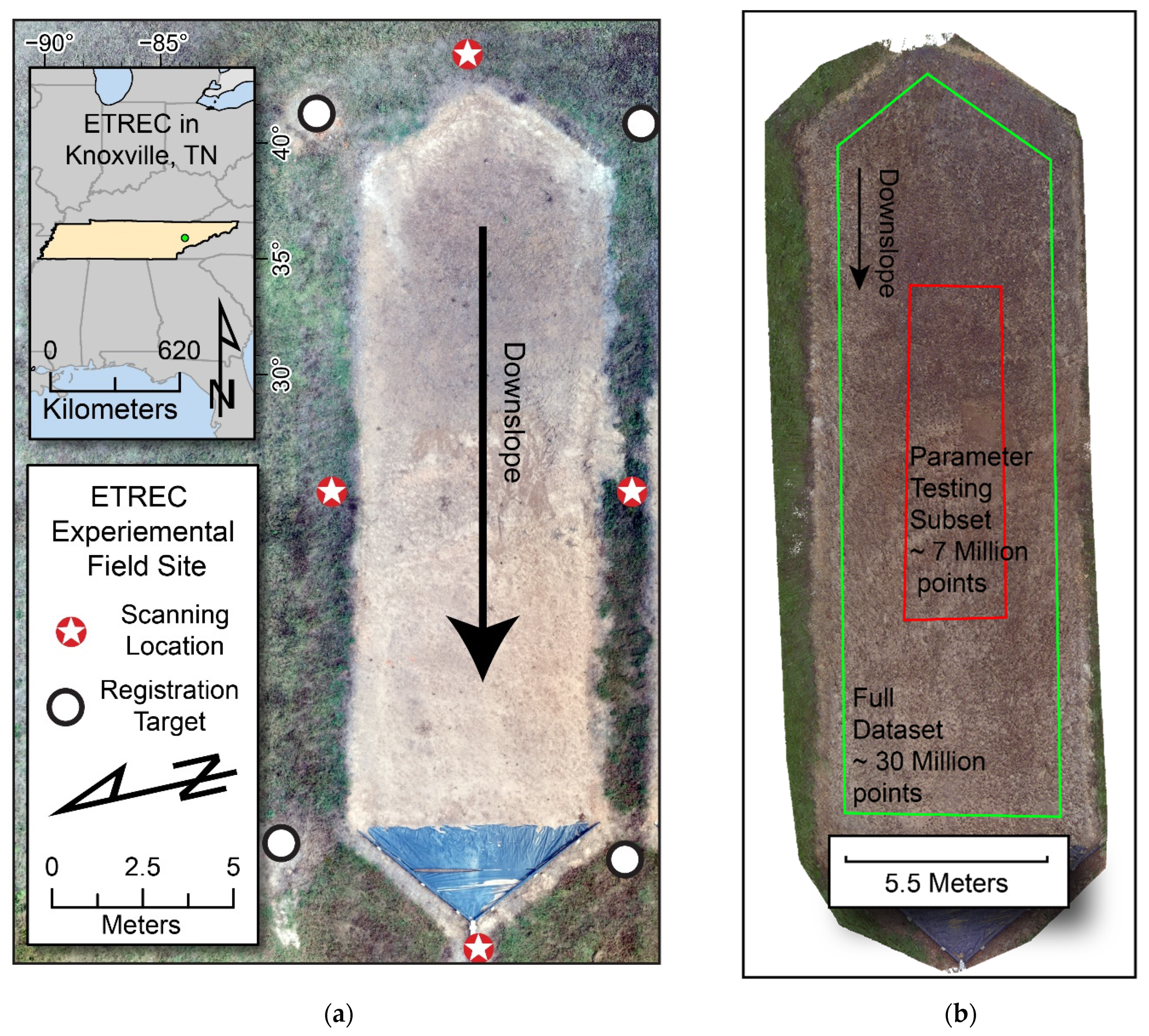
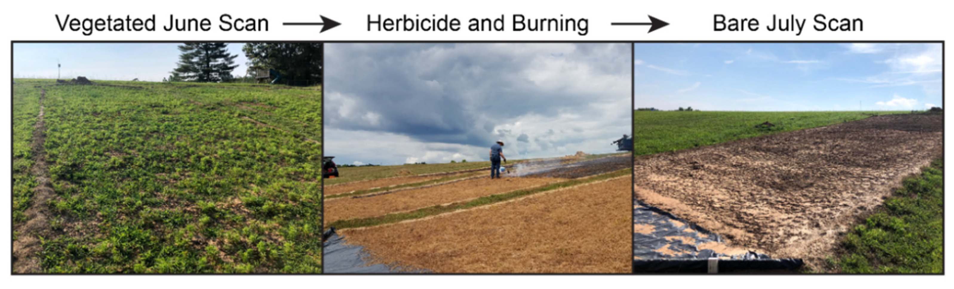
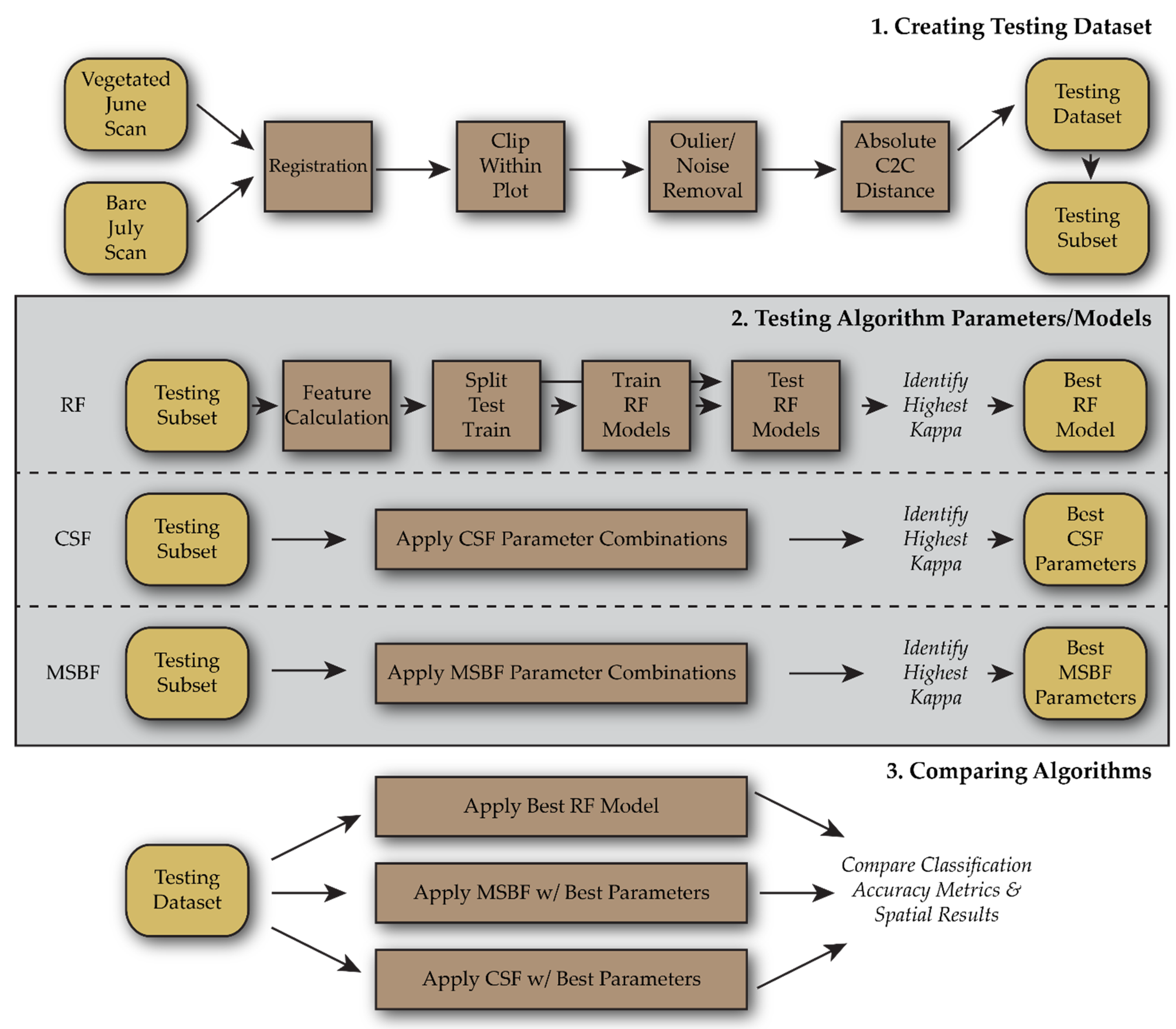
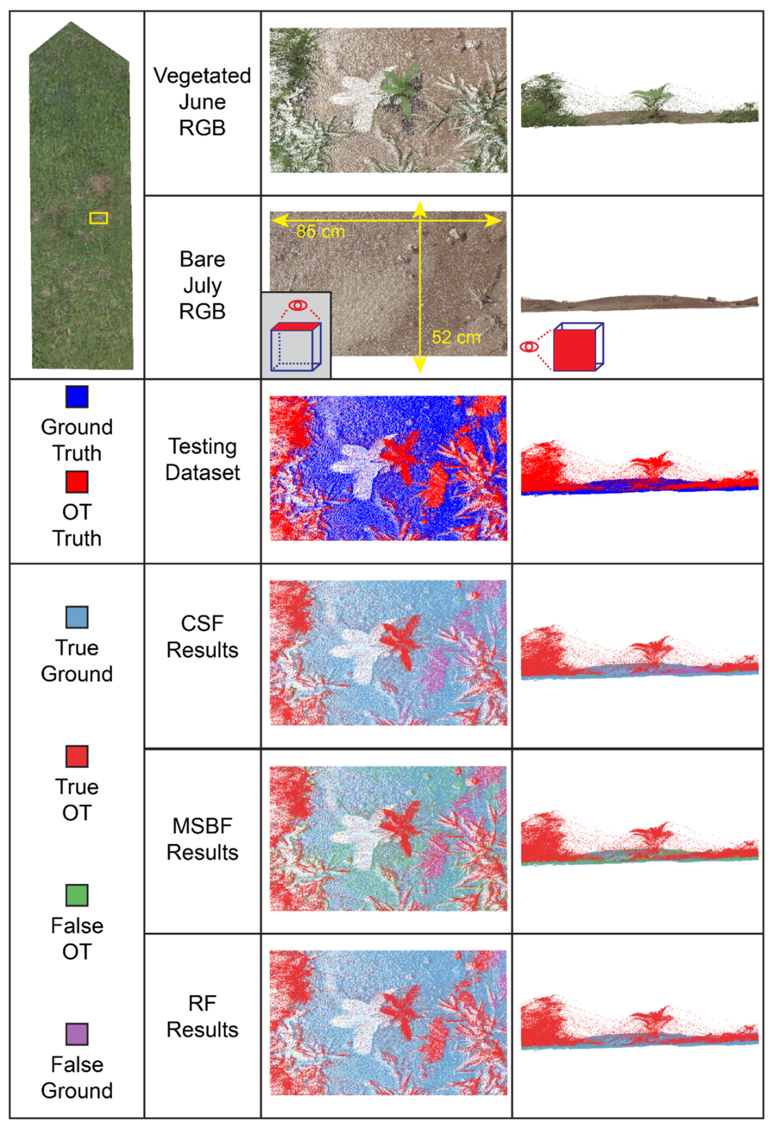
This study assesses the performance of three filtering algorithms: CSF, MSBF, and RF, in identifying ground points from a high-density TLS dataset. Successive TLS scans, one scan under highly vegetated conditions and a second under bare conditions, were collected from a controlled erosion plot to produce a testing dataset of classified ground and OT points. This testing dataset was used to tune the algorithm parameters and measure the performance of each filtering algorithm. The following questions are addressed using these results: (1) Can any of the filtering algorithms effectively remove the vegetation points at fine resolutions?; (2) What is the impact of parameter tuning on the performance of each algorithm?; and (3) Which algorithm provides the best performance with the optimized/tunned parameters? This study provides critical insight into the ground point filtering process, which is essential in using TLS to quantify fine-scale topographic changes.

2. Materials and Methods

2.1. Study Area

The study area is an experimental field site located at the Plant Science unit of the East Tennessee Research and Education Center, University of Tennessee (ETREC) (Figure 1). Data were collected from a hillslope plot at the site. The plot has an approximate length of 21 m, a width of 6 m, and a slope of 15%. The plot is designed to be hydrologically isolated from other parts of the hillslope, with raised berms at the top and sides of the plot and a sediment capturing installation at the bottom. The plot was used for testing the detection limit of TLS on bare hillslope erosion [29], so it was established to be largely free of vegetation with the application of herbicide, allowing time for vegetation to die off and burning off all remaining residues. Photographs demonstrating this process can be seen in Figure 2. The plots underwent no physical disturbance during these processes nor for the ten prior years, so the soil surface elevation should not have been measurably affected.

2.2. Research Design and Filtering Algorithms

Figure 3 shows a flowchart of the whole research design. A test dataset of classified 3D point clouds is needed to assess the performance of different filtering algorithms and the impact of filtering parameters. Several studies have classified points manually, but it is time-consuming and labor-intensive [27,28,30]. In this study, successive TLS scans were collected from the studied plot. One scan was conducted under densely vegetated conditions, and the second scan was conducted about a month after the first scan under bare conditions after removing vegetation. This experiment presents a chance to capture the same plot under different vegetation conditions in a short period without significant surface erosion. These two scans are processed to produce the testing dataset to evaluate if the vegetation points can be effectively removed by filtering algorithms, assess the impact of parameter tuning on vegetation removal for each filtering algorithm, and compare the best performance of different filtering algorithms.
Three automatic filtering algorithms were selected and applied to the testing dataset: Zhang et al.’s [25] inverted cloth simulation filter (CSF), Vosselman’s [26] modified slope-based filter (MSBF), and a random forest (RF) classifier. These algorithms were selected because they are freely available, can be implemented programmatically, and operate only on the positional information of the 3D point cloud (X, Y, Z).
CSF is a surface-based classifier designed for airborne LiDAR that can be conceptualized as a cloth falling over an inverted 3D point cloud. Places touching or within a threshold of this cloth are classified as ground, and the remaining points are classified as OT points. CSF’s input parameters include: (1) ‘smoothing’, a Boolean variable controlling if steep slopes are normalized; (2) ‘cloth resolution’, controlling the grid resolution of the simulated cloth; (3) ‘rigidness’, the rigidity of the simulated cloth; (4) ‘time step’, affecting the displacement of simulated cloth particles during each iteration; (5) ‘classification threshold’, the threshold used to classify the point cloud based on the distance to the simulated cloth, and (6) ‘iterations’, controlling the maximum iterations of the algorithm. A detailed description of the algorithm is given by Zhang et al. [25]. The CSF filter has been implemented in python and MATLAB and is included with the CloudCompare software (https://www.danielgm.net/cc/, accessed on 2 August 2022) as a plugin. For this study, CSF is applied through python Anaconda binaries.
MSBF is a conventional morphology and slope-based technique that uses a white top-hat transformation to equalize ground elevation differences between points before analyzing the slope and height between a point and its neighbors. Points exceeding a set height and slope threshold within a neighborhood are classified as OT points and the remaining points as ground. Adjustable parameters for the MSBF algorithm are: (1) ‘radius’, the radius for a point’s neighborhood; (2) ‘minimum neighbors’, the minimum number of points of a neighborhood; (3) ‘slope threshold’ and ‘height threshold’, the slope and height thresholds for a point to be classified as an OT point relative to its neighbors; and (4) ‘slope normalization’, controlling if slope normalization is performed. A detailed description of the MSBF algorithm is given by Vosselman [26]. This algorithm is available through WhiteBoxTools with command-line tools, a python library, and software implementations [31]. The python implementation is used in this study.
The RF classifier is a supervised machine learning algorithm that classifies points based on a ‘forest’ of decision trees built automatically from relationships between identified features in training data. The RF classifier can be tuned with hyperparameters. Similar to Weidner et al. [27], this study deviates from default settings by using 100 trees with a maximum tree depth of 1000. RF training data are composed of features used to predict labels. The OT points classified in the testing dataset make up the labels for this study. The features used to predict the labels are the three normalized eigenvalues calculated at each point, considering all points within a neighborhood radius of 0.005 m, 0.0075 m, 0.01 m, 0.015 m, and 0.025 m. This results in five features for each neighborhood, for a total of fifteen features considering five spatial scales. The eigenvalues were normalized by dividing a given eigenvalue by the sum of all three eigenvalues for the considered neighborhood radius. Two models were built and tested on a subset of the testing dataset. The first model considered the full range of neighborhood eigenvalues, and the other model only the 0.005 m, 0.01 m, and 0.015 m neighborhood eigenvalues. Conceptually, this should allow the classifier to consider the shape of the surface at slightly different scales. Eigenvalues were calculated using CloudCompare command-line tools. The points within a subset of the testing dataset were randomly split 75/25% for training and testing purposes in building and comparing the two models. The RF classifier was implemented using the sklearn python library [32].
While CSF and MSBF require input parameters, the implementation of the RF classifier requires defined features from testing data to set internal parameters. To examine the influence of different parameters for CSF and MSBF, several hundred combinations of a range of parameters were applied to a subset of the testing dataset on the central portions of the plot (Figure 1b). The same subset was also used as training data to build the RF models. The subset of the testing dataset contains approximately 7 million points, with 2.8 million points classified as ground and 4.2 million points classified as OT points. A subset of the testing dataset was used for analyzing parameters and building the RF classifier to significantly reduce computation time when exploring parameters.

2.3. Data Collection, Registration, and Preprocessing

Two TLS surveys were conducted on 4 June 2020 (June scan) and 6 July 2020 (July scan). The June scan captured plot conditions before removing vegetation and contains dense live and dead, standing and flat vegetation on the plot. The July scan was conducted under bare plot conditions after vegetation was almost completely removed through herbicide killing and burning of standing and surface residue. All scans were collected using a FARO Focus3D X 330 (Faro Technologies, Lake Mary, FL, USA). This scanner has a laser wavelength of 1.55 × 10⁻⁶ m, a beam divergence of 0.00019 rad, and a beam diameter at exit of 0.00255 m. The scanner is rated to measure the distance to surfaces from 0.6 m to 130 m with a ranging error of ±0.002 m at 20 m. The device’s field of view is 360° horizontal and 300° vertical. The scanner is mounted on an extending tripod to gain a favorable scanning angle. After an approximate alignment of the tripod, the scanner’s internal dual-axis compensator levels the scan data with an accuracy of 0.015°. A scanning resolution of 0.5 of the scanner’s full capability is used to balance the density of points with scan time, which results in over 177 million points over the entire field of view with an average point density of 93,000 points/m2 within 20 m and a scan time of roughly 8 min. Scans were collected with the scanner at the top, bottom, and sides of the plot to gain a more even distribution of point densities and a greater likelihood of points reaching the ground (Figure 1). Each scan renders a 3D point cloud file that reports each point with geometric fields (X, Y, Z), color fields (R, G, B), and return intensity.
To control the quality of the TLS data collection, concrete mounting piers were installed at the corners of the plot to serve as permanent and fixed locations for registration targets. Considering the capacity of TLS in delineating 3D shapes, identical spherical registration targets with a diameter of 0.139 m were used. Raw TLS scans were registered using Leica Cyclone software. After importing, the spherical registration targets were manually identified. All eight scans were registered into a single local coordinate system using only the identified spherical targets. For each spherical target, the registration software creates target constraints pairing that target to the same target in every other scan. The registration process attempts to minimize the distance between all target constraints. The quality of registration is assessed through the absolute error, any remaining distance, between valid registration target constraints after registration. A box plot of all absolute errors between target constraints is shown in Figure 4. The registration software reported a mean of the absolute error between target constraints of 0.0035 m. Please check Fan et al. [33] for the details in calculating registration errors. Individual viewpoint scans for the plot at each date were merged into one 3D point cloud. The 3D point cloud is then manually clipped to include only points within a boundary about a half meter away from the plot edge to avoid potential edge effects and reduce the size of the data before further processing (Figure 1b). To remove outlier and noise points, the ‘statistical outlier filter’ tool in CloudCompare was applied to the 3D point clouds. This tool removes any point whose distance, considering a neighborhood of the nearest 50 points, was two standard deviations higher than the average distance between points within the neighborhood.
Assuming that the June and July scans measured the same surface with and without vegetation, any point within the vegetated June 3D point cloud whose distance away from the nearest point in the bare July dataset is greater than the registration error could be reasonably classified as an OT point. However, removing vegetation from the plot took around a month, and the plot did experience some surface erosion during this time. The weather station at the McGhee Tyson Airport, 9.5 km away, recorded 98.2 mm of precipitation between the June and July scan. While the vegetation and residue were still present on the plot until just before the July scan, providing some protection of the surface, it can be assumed that the plot did experience some degree of erosion. To account for this, the threshold distance between points in the vegetated June and bare July clouds used to classify OT points was set to 0.01 m after visual inspection (Figure 5). This distance is considered sufficiently far that the great majority of points in the vegetated June 3D point cloud that are at least 0.01 m away from the bare July 3D point cloud and thereby classified as OT points are a result of genuinely representing a non-ground object rather than a result of noise or an eroded surface. The distances between 3D point clouds were calculated using the cloud-to-cloud (C2C) absolute distance tool within the CloudCompare software, which computes an unsigned distance between every point in one 3D point cloud and the nearest point in another 3D point cloud. After running the C2C tool on the vegetated June and bare July scans, a binary field was generated for the vegetated June 3D point cloud to classify each point as ground or OT based on the C2C absolute distance. This classification is treated as the ‘ground truth’ for further assessment of the performance of the filtering algorithms.

2.4. Performance Assessment Methods

The performance of each filtering algorithm was analyzed using a set of classification accuracy metrics, including overall accuracy, F1-score, recall, and precision. Excluding overall accuracy, the accuracy metrics are defined in the following equations using the terms of a binary classification confusion matrix: true positive ( T P ), true negative ( T N ), false positive ( F P ), and false negative ( F N ) . Precision, P , is defined as the ratio of correct positive classifications to all positive classifications (Equation (1)).
P = T P T P + F P
Recall, R, is defined as the ratio of correct positive classifications to all true positives (Equation (2)).
R = T P T P + F N
The F1-score, F1, is the harmonic mean of precision and recall (Equation (3)).
F 1 = 2 × P × R P + R
F1-score, recall, and precision are reported for both OT and ground classes. In addition, Cohen’s Kappa score, k, is calculated and used as the primary metric for analyzing parameter performance and overall model performance (Equation (4)).
k = 2 × ( T P × T N F N × F P ) ( T P + F P ) × ( F P + T N ) + ( T P + F N ) × ( F N + T N )
Cohen’s Kappa considers the possibility of agreement occurring by chance among raters [34] and is more robust to imbalances in the dataset. Unlike F1-score, recall, and precision, it provides a single agreement value that considers both classes. McHugh [35] suggests Cohen’s Kappa scores above 0.6 indicate a ‘Moderate’ agreement, scores above 0.8 a ‘Strong’ agreement, and scores above 0.9 an ‘almost perfect’ agreement.
Considering the immense dataset size and the challenges of displaying three-dimensional data, we illustrate the classified points using three smaller sites within the plot representing a range of conditions and a cross-sectional profile across the middle of the plot. At each site, the 3D point cloud is viewed from two perspectives. A top-down perspective compresses the Z (height) axis, highlighting the X (side-to-side) and Y (up-and-down slope) axes. A side view looking upslope compresses the Y axis, showing the X and Z axes. At each site and from each perspective, the colors of the points in the 3D point cloud are used to visualize site conditions, testing data, and algorithm results. The testing dataset classifications and RGB points from the bare and vegetated scans provide context for the surface. The results from each algorithm are shown using four classes. ‘True Ground’ and ‘True OT’ are points correctly classified as ground or OT. ‘False OT’ is a ground point in the testing dataset that the algorithm classified as OT, and ‘False Ground’ is an OT point in the testing dataset classified as ground by the algorithm. The same four classes are also used to illustrate the cross-sectional profile across the middle of the plot.

3. Results

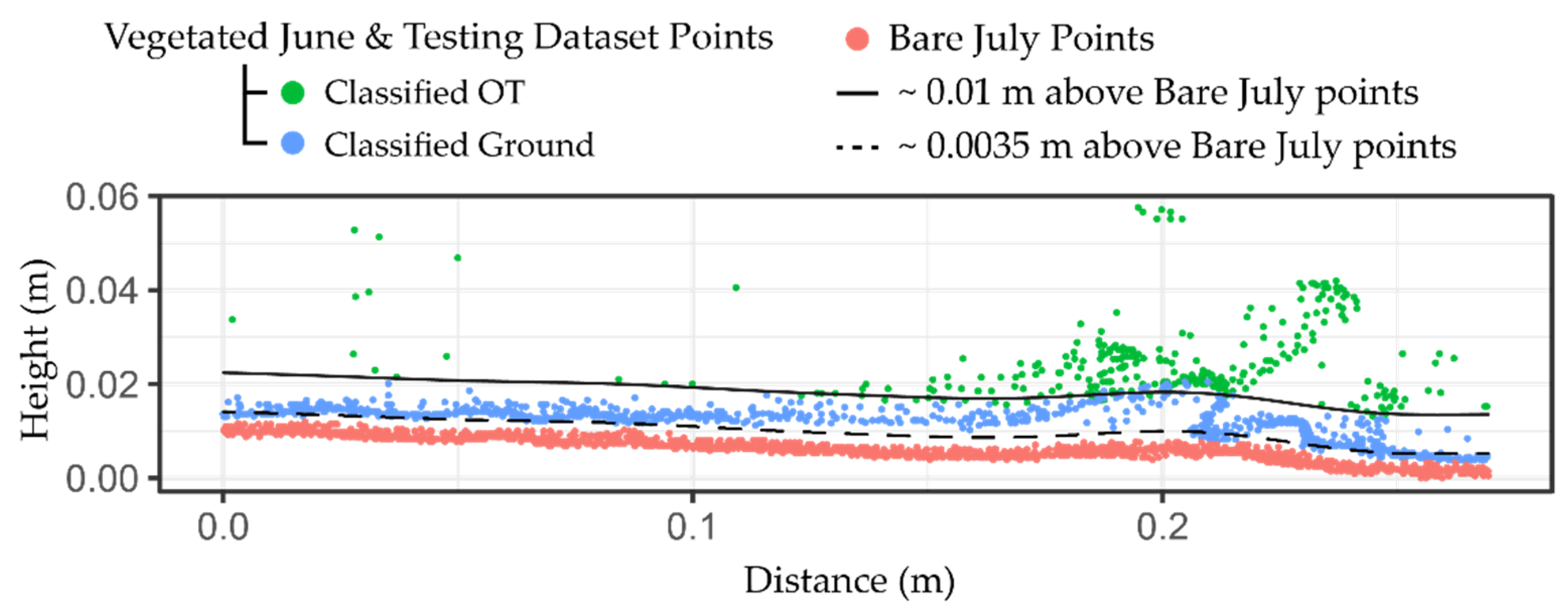
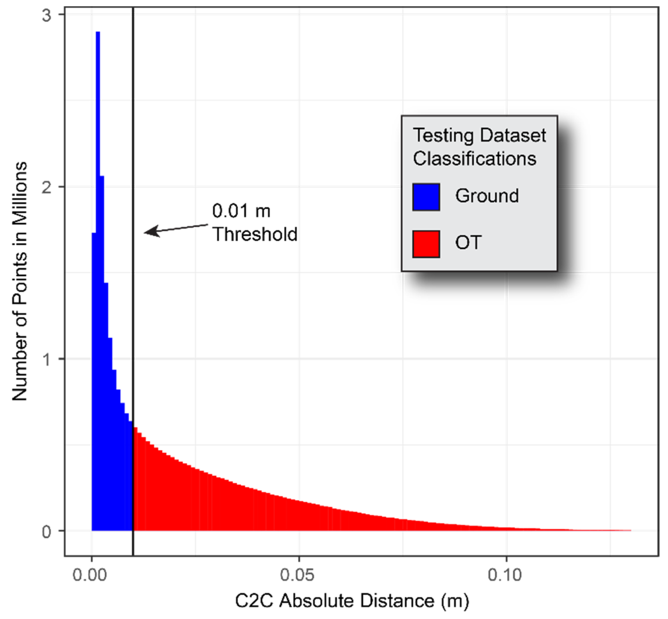
Of the over 30 million points, approximately 13 million points had a C2C absolute distance of <0.01 m between the vegetated June and bare July scans, and 17 million points had a C2C absolute distance of >0.01 m. These points are classified as ground and OT points, respectively. 
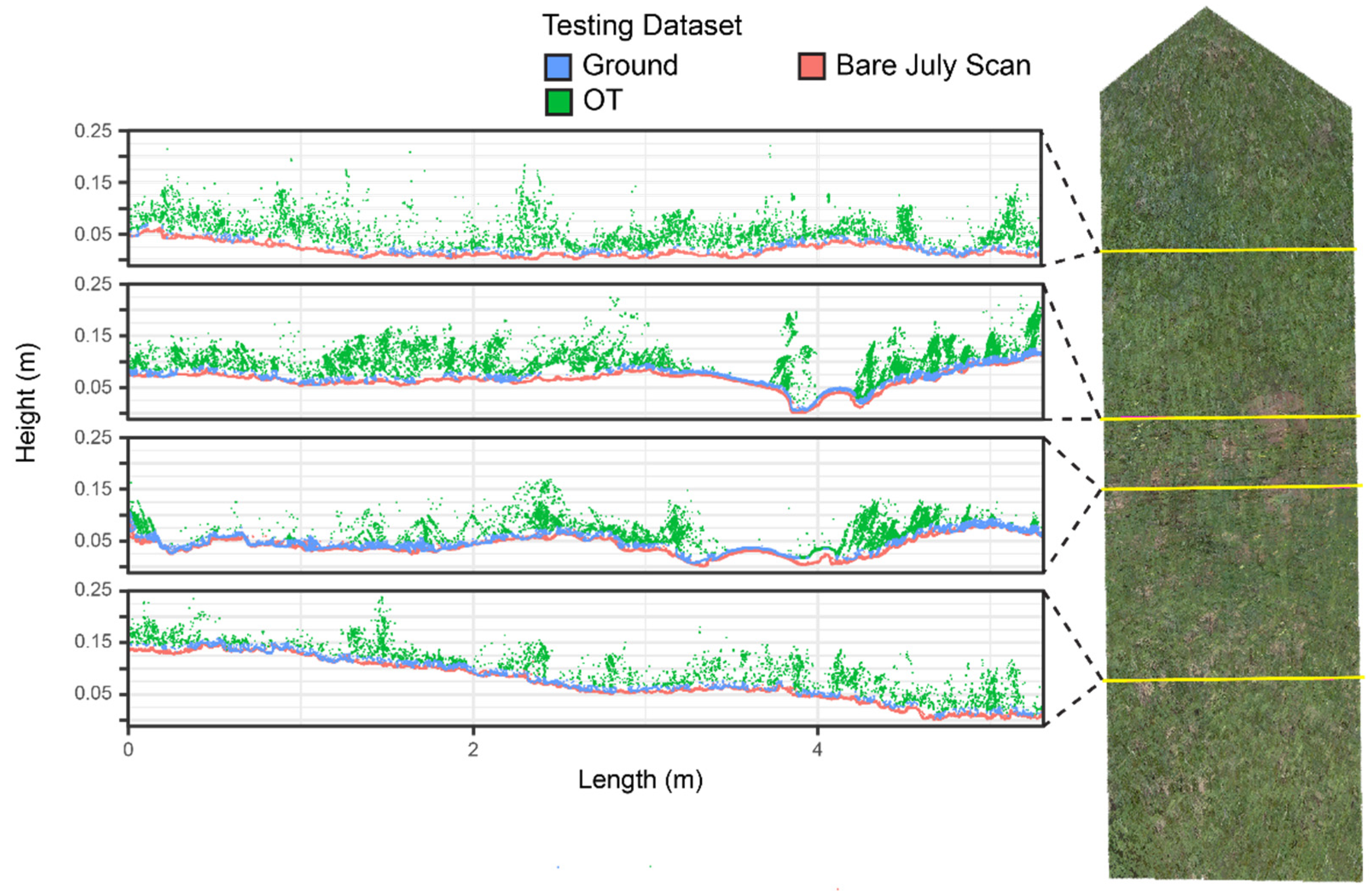
Figure 6 shows the histogram of the C2C absolute distances and classifications. Cross sections of the testing dataset overlaying the bare July 3D point cloud reveal a close agreement between the ground classified points and the points from the bare scan where vegetation is sparse (Figure 7). In highly vegetated areas, fewer points fall under the 0.01 m threshold, and ground-classified points occur much more infrequently.
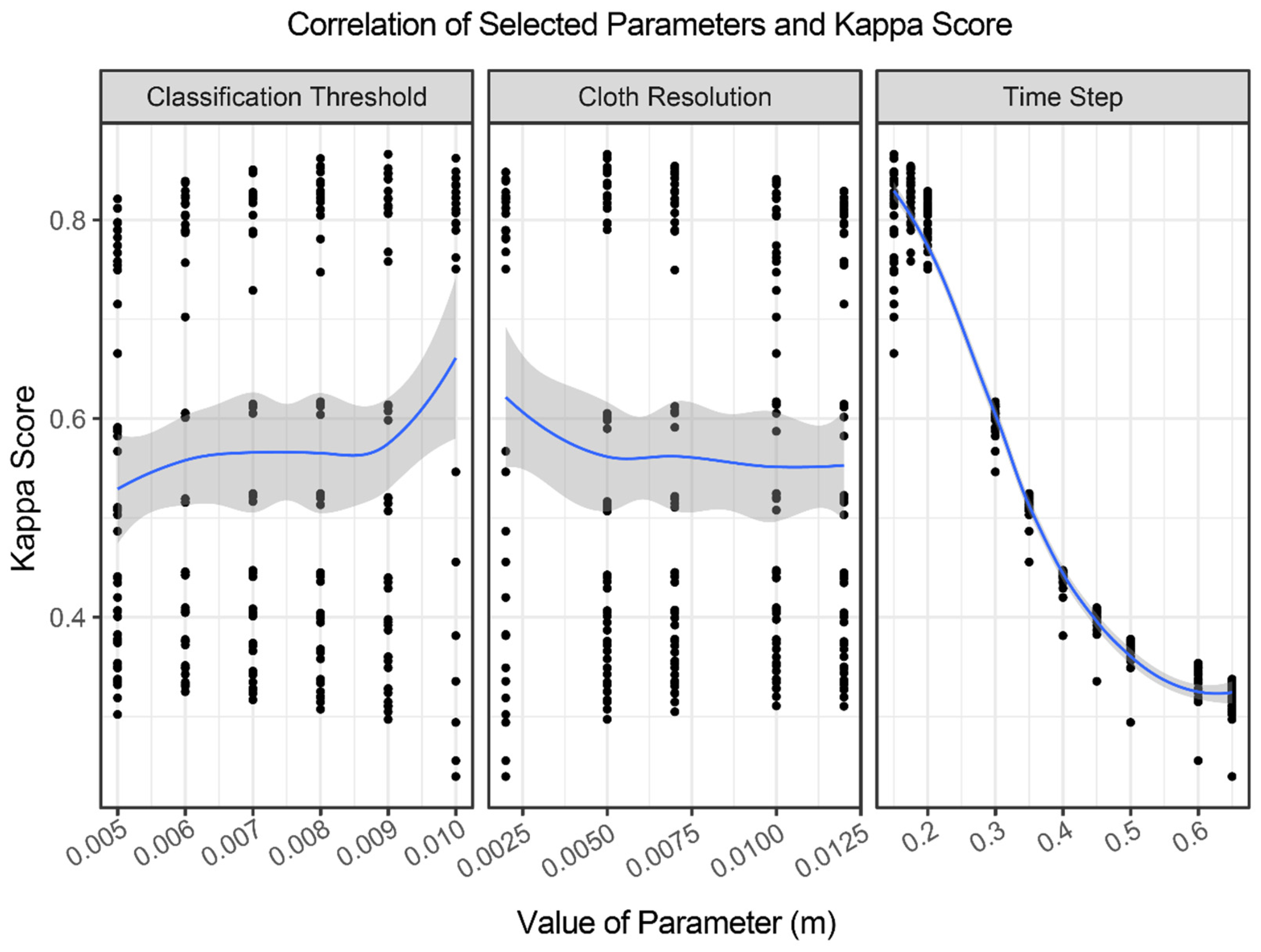
The adjustable parameters of the CSF algorithm are ‘smoothing’, ‘cloth resolution’, ‘rigidness’, ‘time step’, ‘classification threshold’, and ‘iterations’. Of these parameters, only ‘cloth resolution’, ‘time step’, and ‘classification threshold’ were found to substantially affect the classification. The parameters that did not affect classification were set to the recommended default values of ‘smoothing = false’, ‘rigidness = 3’, and ‘iterations = 500’. For the parameters affecting the classification, combinations of the following value ranges were used: ‘cloth resolution’ from 0.002 m to 0.012 m; ‘time step’ from 0.1 m to 0.65 m; and ‘classification threshold’ from 0.005 m to 0.01 m. This resulted in 277 combinations of parameters being applied to a subset of the testing dataset. These values were selected considering the point density of the dataset and the expected scale of changes.
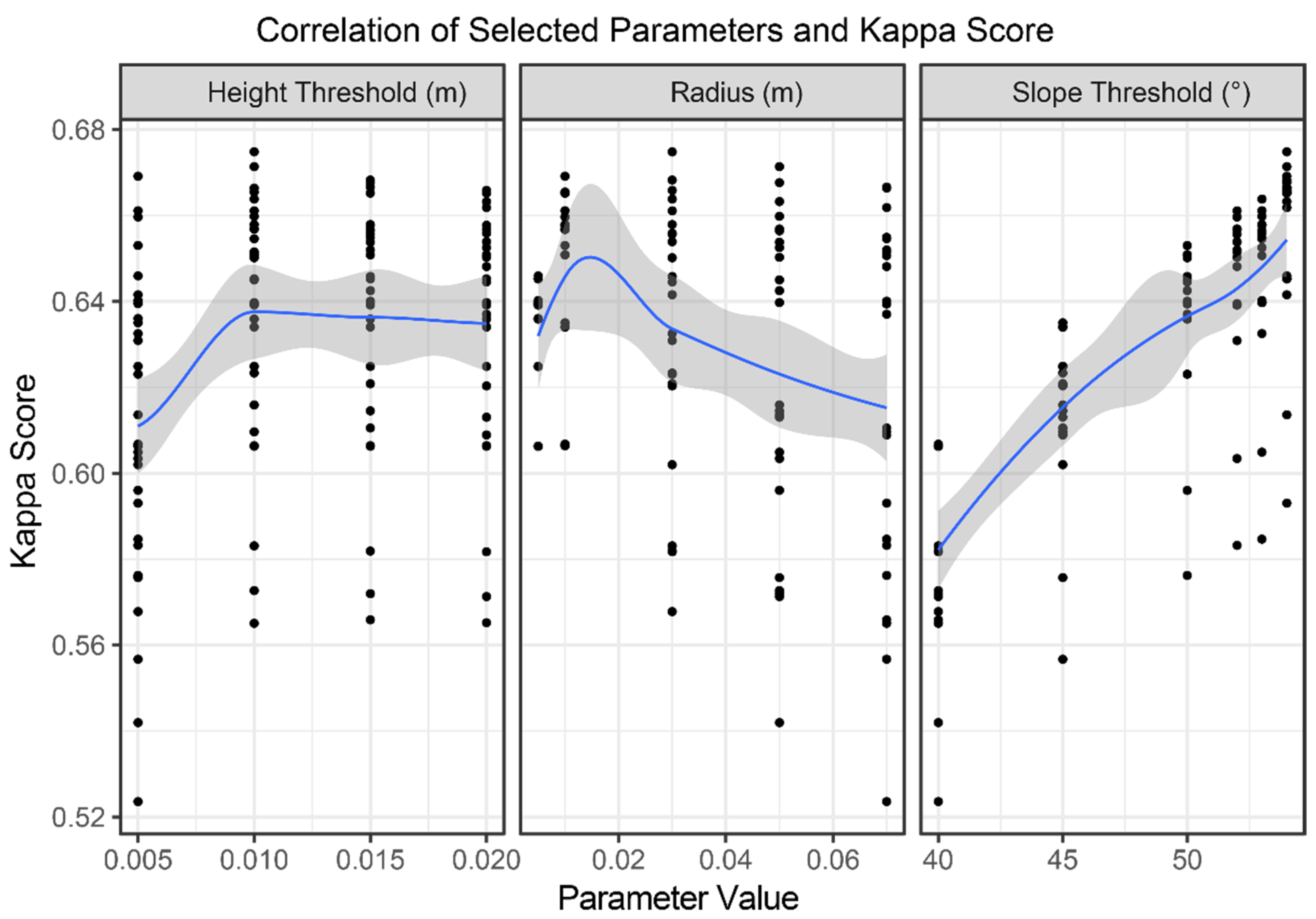
For the MSBF algorithm, combinations of input parameters of the following value ranges were used: ‘radius’ from 0.005 m to 0.07 m; ‘minimum neighbors’ from 10 to 75; ‘slope threshold’ from 40° to 54°; ‘height threshold’ from 0.005 m to 0.02 m; and ‘slope normalization’ at True or False. This total of 721 combinations were applied to a subset of the testing dataset. Like CSF, considering point density and surface topography, these values were selected as reasonable inputs.
Nearly 1000 iterations of input parameters for the CSF, MSBF algorithms, and two variations of RF models are applied to the subset of the testing dataset. The highest performing CSF parameter iteration resulted in a Kappa value of 0.86, with the lowest iteration resulting in a Kappa score of 0.24. Iterations of the CSF parameters where the ‘time step’ parameter was below 0.15 m resulted in a failed classification. Of the impactful CSF parameters, the ‘time step’ parameter was most strongly correlated with the Kappa score and appears to be the primary driver of algorithm performance (Figure 8). The sets of input parameters that produced the highest Kappa value are given in Table 1 and are further applied to the entire dataset.
The parameter iterations of the MSBF algorithm applied to the subset dataset produced a tighter range of Kappa values from 0.67 to 0.52. For this dataset, the ‘Slope Threshold’ parameter had the closest correlation with algorithm performance (Figure 9). The parameters producing the highest Kappa value are listed in Table 1, and these parameters were applied to the entire testing dataset.
The performances of the two RF models were compared for the subset dataset using a randomly generated 75% and 25% of points for model training and testing, respectively. Relative to the 25% of points from the subset, the RF model built considering the eigenvalues of five neighborhood scales outperformed the model built on three scales in all metrics. The inclusion of two additional neighborhood scales, 0.0075 m and 0.025 m, into the model’s base training dataset of 0.005 m, 0.01 m, and 0.015 m increased the Kappa value from 0.63 to 0.72. The RF model built using the full range of neighborhood scales was then applied to the entire dataset (including all points within the subset).
Only the optimal parameters/models were used for the whole testing dataset to evaluate the performances of CSF, MSBF, and RF approaches (Table 2). The CSF algorithm outperforms the other algorithms in most metrics except the ground precision and OT recall, for which MSBF narrowly outperformed CSF. The accuracy metrics for CSF and RF are balanced between the ground and OT classes, with CSF scoring slightly higher in every category.
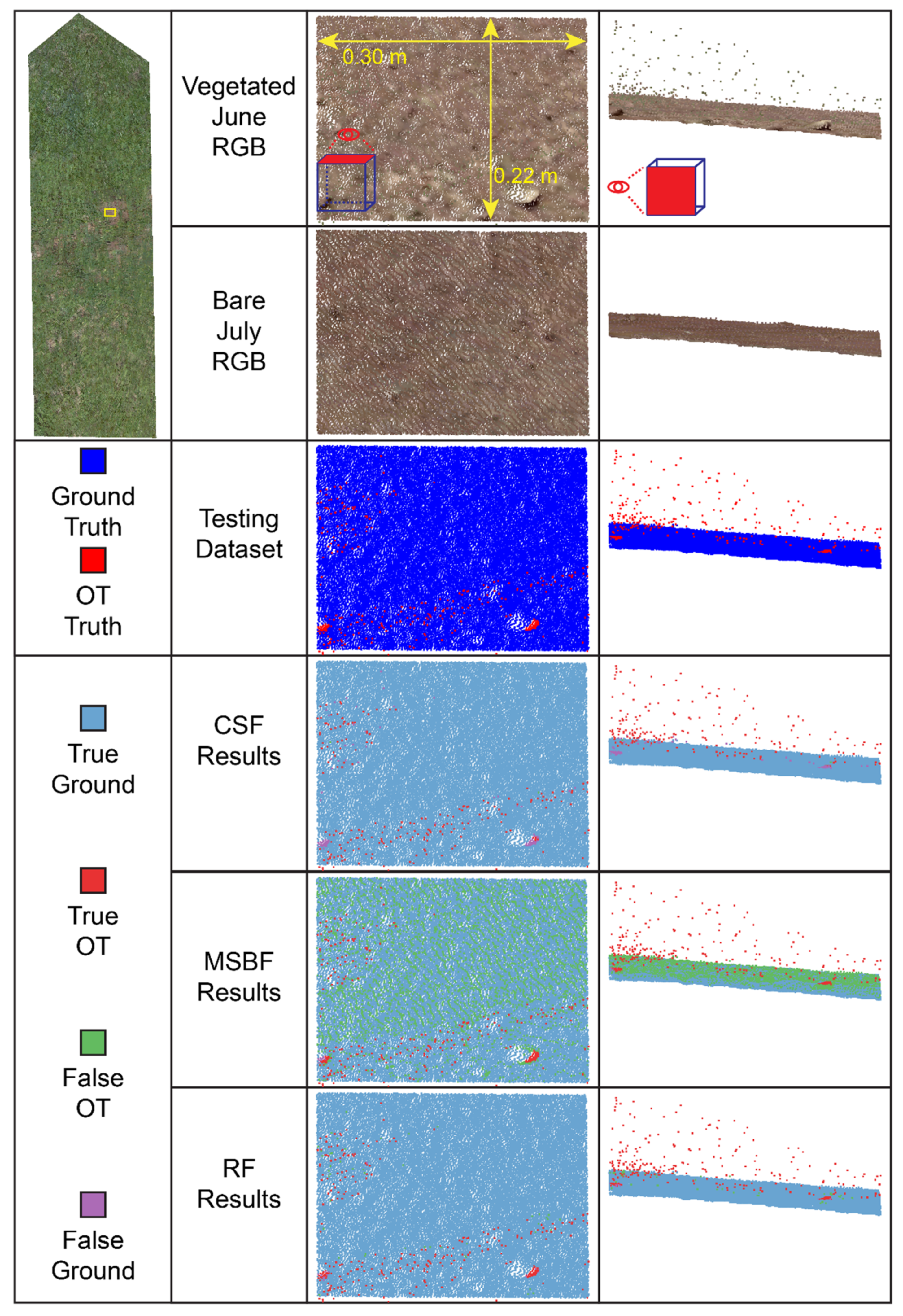
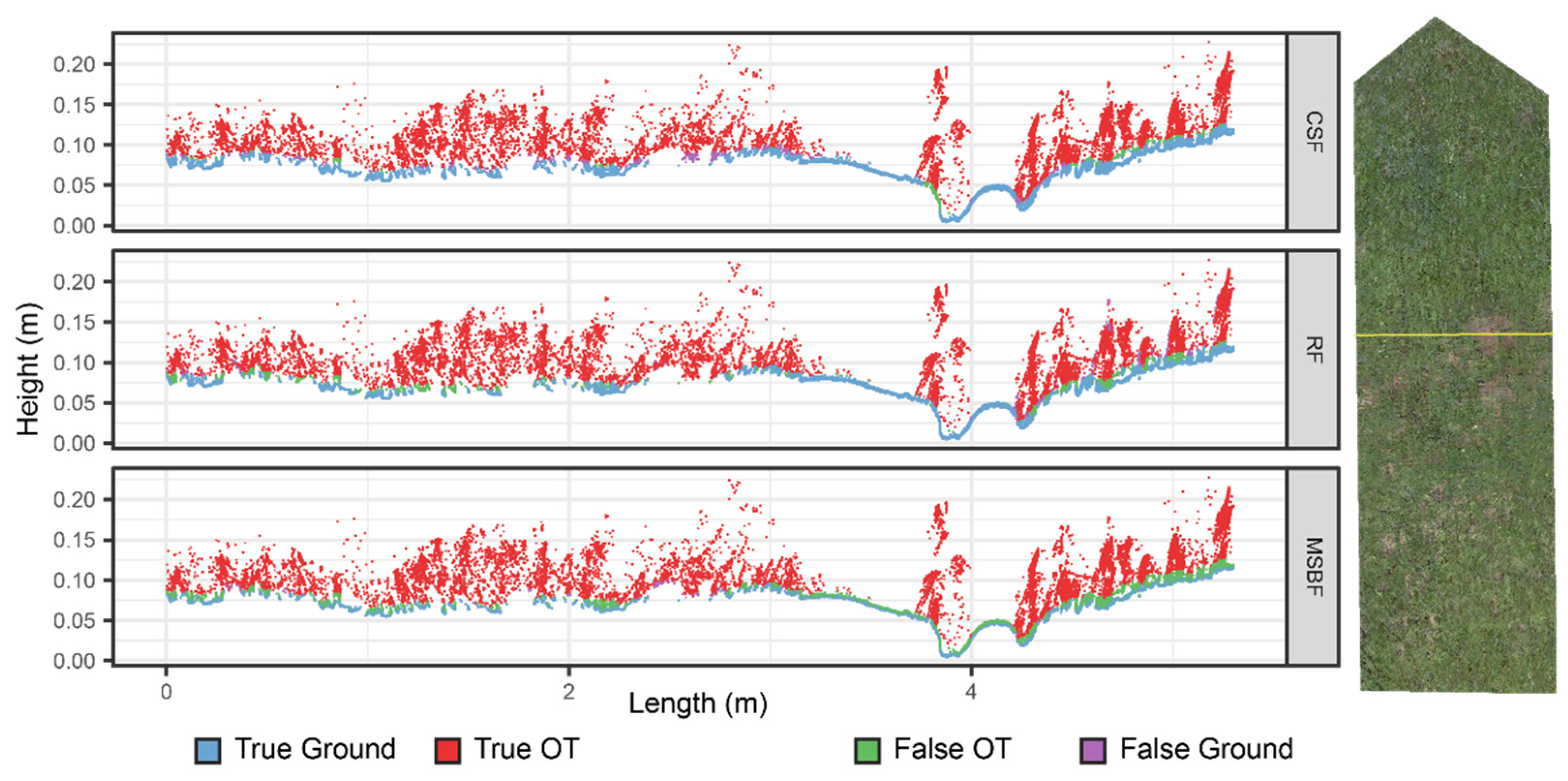
Figure 10 shows a portion of the plot free of vegetation. At this location, the few OT points of the testing dataset result from noise reflections and portions of a small pebble that moved into the area between scans. All algorithms easily identify these OT points. The only noticeable difference is with the MSBF, which consistently falsely classifies OT points over most of the surface. The cross-section results also show this pattern for MSBF (Figure 11): along the correctly classified ground points, there is a layer of falsely classified OT points that is not present for the other algorithms.
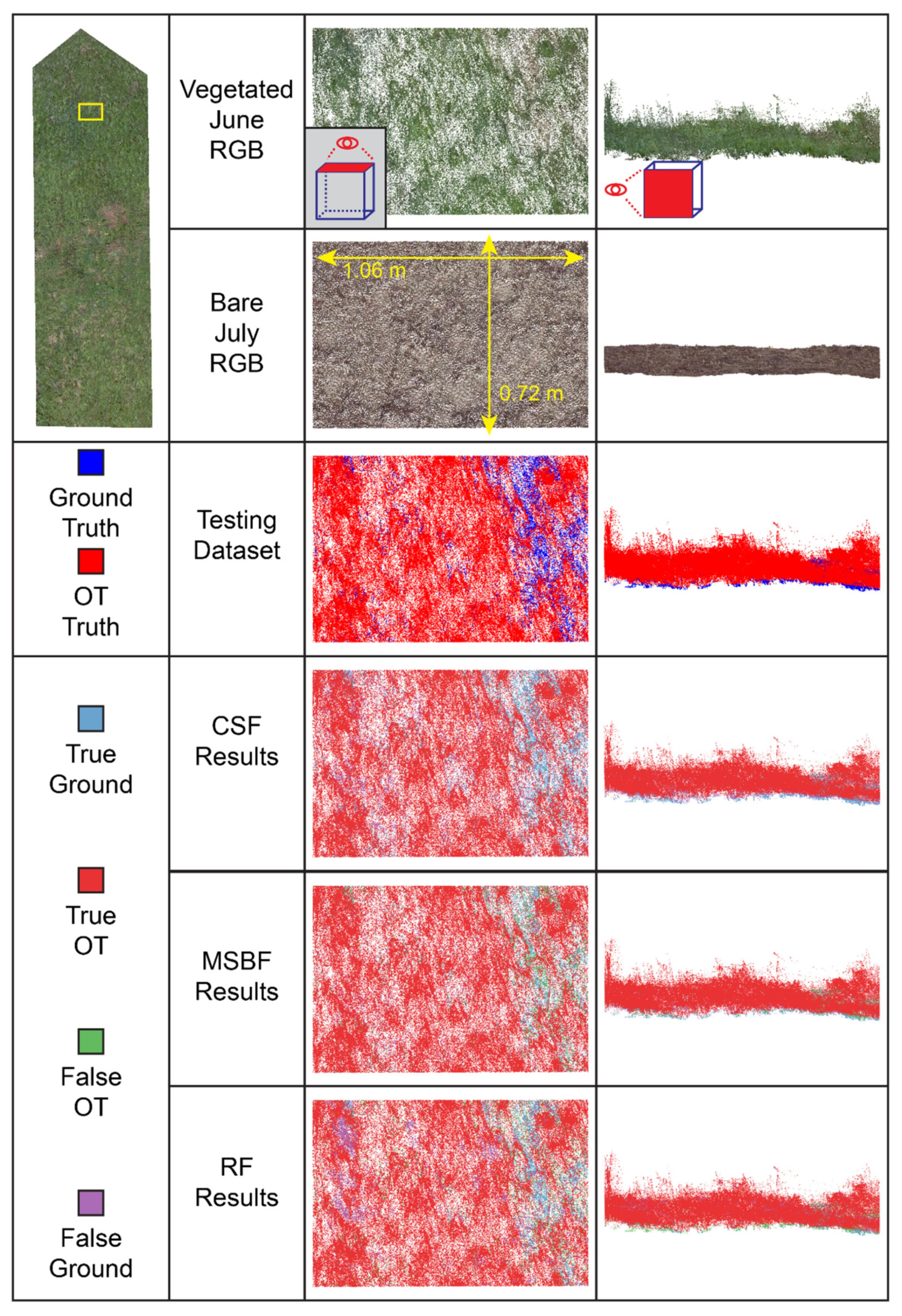
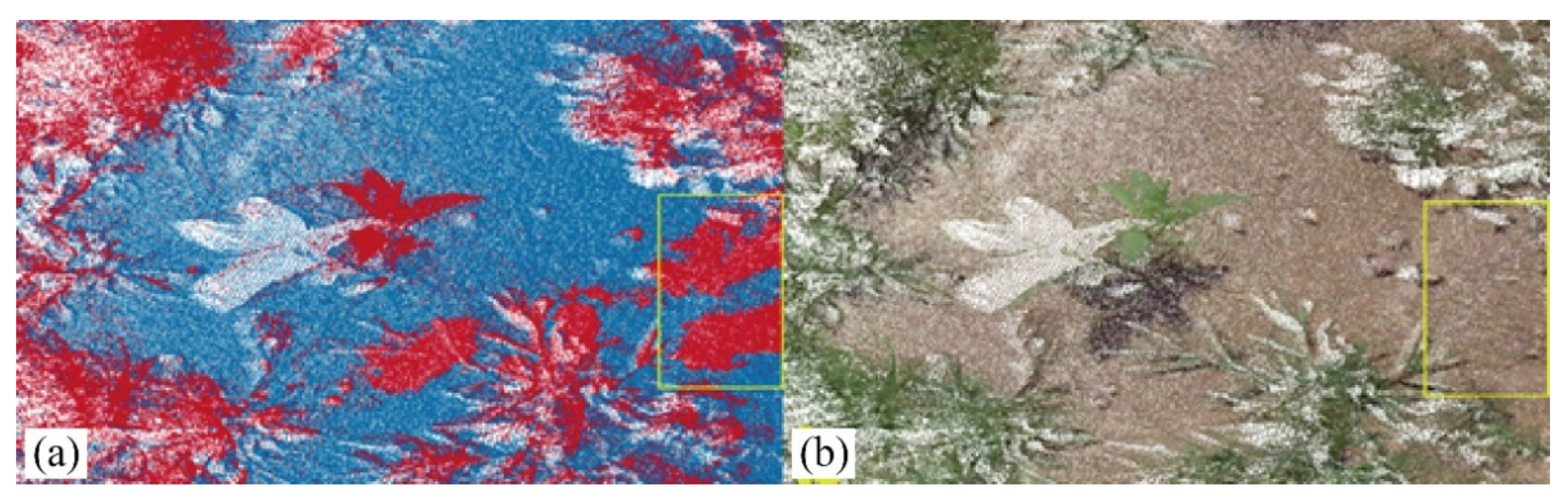
Figure 12 shows a portion of the plot dominated by vegetation. At this site, CSF is remarkably accurate relative to the other algorithms. CSF falsely classifies some OT points as ground on the left portions of the site where the vegetation is thicker but to a lesser degree than RF. The RF classifier misclassifies points more frequently than the other algorithms in densely vegetated areas. The MSBF’s high OT recall score suggests that the MSBF excels in this vegetated area, although the same pattern of disqualifying many ground points is still evident on the right portion of the area.
The area shown in Figure 13 contains a variety of conditions: taller, denser vegetation on the left, a single plant surrounded by flat ground in the center, and short vegetation close to ground on the right. The CSF and RF algorithms classify most ground and densely vegetated areas correctly. The MSBF algorithm again shows the pattern of excessively excluding ground points.

4. Discussion

4.1. Testing Dataset

A test dataset is needed to assess the performance of the point filtering algorithms. Studies have generated the testing dataset by manual classification of ground and OT points, which is time consuming and labor intensive [28]. It is also difficult to generate a large and high-density testing dataset using the manual classification approach. The 3D point clouds obtained by terrestrial LiDAR include millions of points, and the point spacing is in millimeters to centimeters.
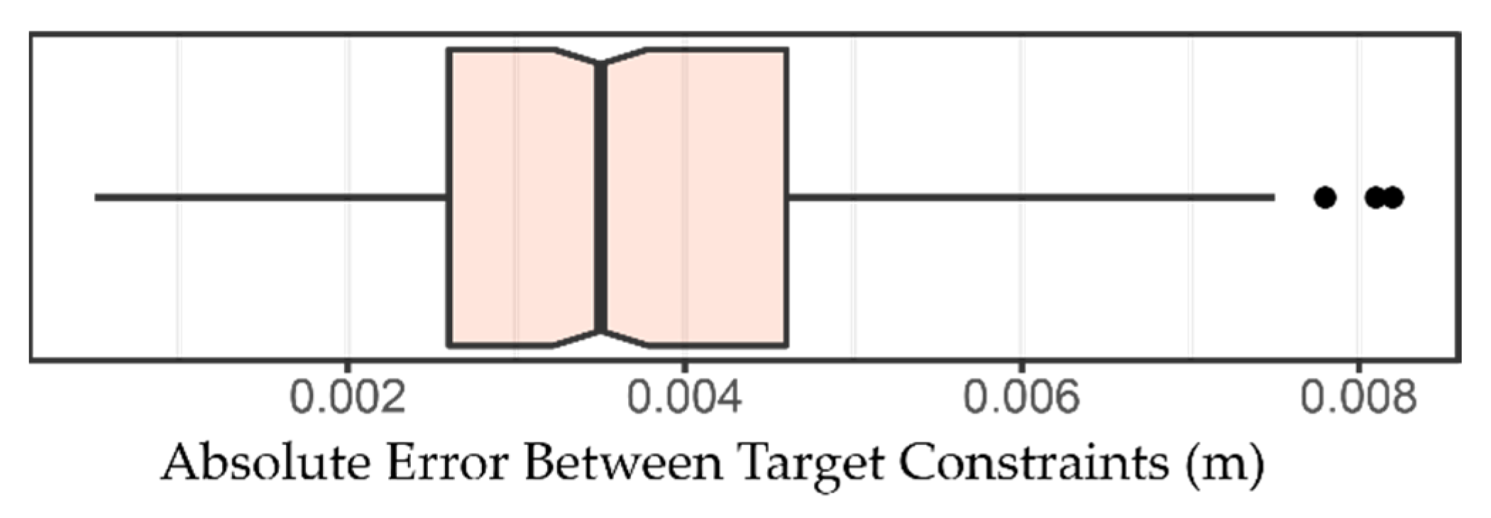
In this paper, we used a novel approach to generate the testing dataset by the comparison of the two successive scans before and after removing vegetation. Assuming no ground surface changes occur during vegetation removal, the C2C absolute distancing between two ground points at the same location would be within two registration errors (0.007 m) of the two 3D point clouds (99% confidence level). However, we did observe some ground surface changes during the one-month period between the two scans. To account for this potential impact, we used a much larger distance of 0.01 m as the C2C absolute distance threshold to classify the testing dataset into ground and OT points (about three registration errors, 99.9% confidence level). This method is fast and efficient, and the created dataset is also large enough for the performance assessment of the filtering algorithms.
However, despite the use of a much larger distance threshold of 0.01 m between the two scans for the point classification, misclassified OT points still exist within the testing dataset. These misclassified OT points are from true ground surfaces that experienced erosion between the two scans. Figure 14 shows an example of the misclassified OT points in the testing dataset. Another example can be seen in the second cross sectional profile from the bottom at the 4 m length mark in Figure 7. It is possible to manually identify and remove errors in the testing dataset. However, it is time consuming and requires a significant effort to check and fix these errors on a complex dataset of many millions of points. In future studies, these errors may be mitigated by either shortening the time between conducting vegetated and bare scans or preventing the experimental plot from being exposed to rainfall between scans. Overall, this misclassification appears rare and is considered an acceptable trade-off to enable the automated classification of the ground and OT points from the 3D point cloud of >30 million points.

4.2. The Impacts of Various Parameters on the Performance of Different Algorithms

Each filtering algorithm uses various parameters for 3D point cloud filtering or classification. However, few studies have examined the impacts of these parameters on the performance of varied types of 3D point clouds. In this study, we identified the most sensitive and the best performance parameters of each filtering algorithm by the comparison of a set of classification results using different combinations of parameters. Our results based on the CSF algorithm directly contrast with the original study of this algorithm for airborne LiDAR, which suggested that a ‘time step’ parameter of 0.65 m was suitable for most situations [25]. For our TLS data, the use of 0.65 m for the ‘time step’ parameter produces the least accurate results, whereas the use of a much smaller ‘time step’ value of 0.15 m achieves the highest Kappa score. It seems that TLS and airborne LiDAR data have dramatically different scales in terms of the ‘time step’ parameter. In addition to the challenges associated with applying CSF to TLS, the simulated cloth used by CSF may ‘stick’ to true OT points whose elevation profile transitions gradually away from the true ground, resulting in a false ground classification. Our results suggest that the CSF algorithm can produce excellent classifications on dense TLS datasets if the input parameters are carefully considered, as the default parameter settings do not seem to apply to high-density TLS point clouds.
Our initial observation of the correlations between individual parameters and the Kappa values for MSBF suggested that the impacts of different parameters are somewhat obfuscated by the interactions between parameters. Future research is needed for a more detailed sensitivity analysis on the impact of the MSBF parameters.
In terms of the RF classifier, the inclusion of additional scales improved the classification results, although a trade-off exists between the benefit of additional scales and increased computation time and complexity. For our test dataset, it appears that the improvement of the Kappa value by 0.09 is worth the computational cost of moving from a 3-neighborhood scale (9 features) to a 5-neighborhood scale (15 features).

4.3. The Comparison of Different Algorithms on 3D Point Cloud Classification

The results based on our testing dataset indicate that CSF outperformed RF and MSBF for the ground and OT point classification of TLS-generated point clouds. CSF scored higher in most metrics, including a Kappa score of 0.86 compared to 0.75 for RF and 0.62 for MSBF when using the best performance parameters. Although CSF was originally designed for airborne LiDAR data, it can produce a highly accurate classification of TLS data when the parameters are carefully considered.
Even with the lowest Kappa score, MSBF produced the highest ground precision and OT recall score, suggesting that it may be advantageous when it is critical to capture only ground points at the cost of excluding some ground points. A closer observation of the MSBF classification results suggests that many falsely classified OT points are slightly above the other ground points in relatively flat areas. This distribution pattern indicates that these points may originate from an individual scanning view farther away from the site. Because these points are less than 0.01 m from the bare surface, they are classified as ground points in the testing dataset. However, MSBF likely classified these points as OT points based on the slope threshold. The application of MSBF to varied surface conditions within a single site may be limited as only a single set of slope and height thresholds are used. Additionally, if OT points are clustered together to create a relatively large and smooth enough surface, the measured neighborhood slope and height may fall below the thresholds, resulting in the misclassification of these OT points to the ground points.
In an area illustrated in Figure 13, both CSF and RF classify most flat ground and densely vegetated areas correctly, whereas MSBF again shows the pattern of excessively excluding ground points. However, this site also contains portions of the testing dataset that are incorrectly classified as OT points because of >0.01 m surface erosion between the two scans. Detailed examination of the classification results suggests that CSF and MSBF classify the ground points more accurately at this site because both methods classify the eroded portions as ground. Interestingly, the RF classifier agrees with the misclassified testing data because of the use of these misclassified points as the training data, suggesting that the RF implementation is sensitive to the training data selection, and even the relatively few errors in our testing dataset may be inappropriate for training RF models. However, our study is only a case study. More work is needed in the future to examine if there are more appropriate surface features that may be used to generate RF models or if the selected features are applicable to a site with different surface characteristics.

5. Conclusions

This study used successive high-density TLS scans of a hillslope plot before and after removing vegetation to generate an automatically classified testing dataset to assess the performance of three point filtering algorithms: CSF, MSBF, and RF. Our results indicate that the performance of each algorithm is affected by the selection of input parameters. The ‘time step’ parameter was highly influential over classification accuracy for the CSF algorithm. The default value recommended by the algorithm in processing airborne LiDAR data leads to the least accurate classifications for these 3D point clouds, whereas a much smaller ‘time step’ value produces the highest classification for TLS data. The variations of parameters for the MSBF algorithm produced a tighter—though less accurate—range of classification accuracies. The ‘slope threshold’ parameter showed the closest correlation with classification accuracy. Two RF models were tested, considering 3 and 5 neighborhoods of eigenvalues, and RF classification accuracy increased with increasing numbers of neighborhoods.
In terms of classification accuracy, CSF outperformed both RF and MSBF. CSF scored higher in most metrics, including a Kappa score of 0.86 compared to 0.75 for RF and 0.62 for MSBF. It is evident that although designed for airborne LiDAR data, CSF can produce a highly accurate classification of TLS data if the parameters are carefully considered. Even with the lowest Kappa score, MSBF produced the highest ground precision and OT recall score, suggesting that it may be advantageous when it is critical to capture only ground points at the cost of excluding some ground points. In addition, a detailed examination of MSBF-classified results displayed a pattern of falsely identifying ground points as OT in locations where the points were slightly above relatively flat areas. RF produced moderate classifications despite being trained using only fifteen features.
This study suggests that the performance of filtering algorithms varies depending on parameter settings. An in-depth sensitivity analysis for different parameter settings may further extend the applications of these filtering algorithms in TLS data. It should be noted that the testing dataset developed in this study is not perfect because the plot experienced some erosion between the two scans. To mitigate the effects of erosion, this study used a larger threshold (0.01 m) than the registration error (0.0035 m) to classify the testing dataset. Despite this, misclassified points can be observed in some sites, and these affected the performance assessment of the filtering algorithms. Future studies may consider applying the filtering algorithms to other well-classified testing datasets obtained by TLS. In addition, the surface characteristics of the experimental plot in this study are fairly homogenous, and the best parameters derived for these filtering algorithms require further testing before being applied to other surfaces where TLS data may require filtering.

Author Contributions

Conceptualization, G.B. and Y.L.; funding acquisition, G.B. and Y.L.; investigation, G.B., Y.L., N.M., D.Y. and W.W.; methodology, G.B., Y.L., D.Y. and H.H.; project administration, Y.L. and D.Y.; resources, Y.L., N.M., D.Y. and W.W.; software, G.B. and Y.L.; visualization, G.B.; writing—original draft, G.B.; writing—review and editing, Y.L., D.Y., H.H., W.W. and N.M. All authors have read and agreed to the published version of the manuscript.

Funding

This research received financial support from the Environmental Protection Agency Small Urban Water Grant (UW-00D45316) and the Carole Anne Shirley Memorial Fund to Y.L., and the Stewart K. McCroskey Memorial Fund to G.B. from the Department of Geography & Sustainability, University of Tennessee. Funding for open access to this research was provided by the University of Tennessee’s Open Publishing Support Fund.

Data Availability Statement

The data related to this study are available on request from the authors.

Acknowledgments

The authors thank Yasin Wahid Rabby and Ming Shen for their help in the field surveys.

Conflicts of Interest

The authors declare no conflict of interest. The funders had no role in the design of the study; in the collection, analyses, or interpretation of data; in the writing of the manuscript, or in the decision to publish the results.

References

  1. Lefsky, M.A.; Cohen, W.B.; Parker, G.G.; Harding, D.J. Lidar Remote Sensing for Ecosystem StudiesLidar, an Emerging Remote Sensing Technology That Directly Measures the Three-Dimensional Distribution of Plant Canopies, Can Accurately Estimate Vegetation Structural Attributes and Should Be of Particular Interest to Forest, Landscape, and Global Ecologists. BioScience 2002, 52, 19–30. [Google Scholar] [CrossRef]
  2. Tarolli, P. High-Resolution Topography for Understanding Earth Surface Processes: Opportunities and Challenges. Geomorphology 2014, 216, 295–312. [Google Scholar] [CrossRef]
  3. Tarolli, P.; Dalla Fontana, G. Hillslope-to-Valley Transition Morphology: New Opportunities from High Resolution DTMs. Geomorphology 2009, 113, 47–56. [Google Scholar] [CrossRef]
  4. Slatton, K.C.; Carter, W.E.; Shrestha, R.L.; Dietrich, W. Airborne Laser Swath Mapping: Achieving the Resolution and Accuracy Required for Geosurficial Research. Geophys. Res. Lett. 2007, 34, L23S10. [Google Scholar] [CrossRef]
  5. Eltner, A.; Baumgart, P. Accuracy Constraints of Terrestrial Lidar Data for Soil Erosion Measurement: Application to a Mediterranean Field Plot. Geomorphology 2015, 245, 243–254. [Google Scholar] [CrossRef]
  6. Lu, X.; Li, Y.; Washington-Allen, R.A.; Li, Y.; Li, H.; Hu, Q. The Effect of Grid Size on the Quantification of Erosion, Deposition, and Rill Network. Int. Soil Water Conserv. Res. 2017, 5, 241–251. [Google Scholar] [CrossRef]
  7. Lu, X.; Li, Y.; Washington-Allen, R.A.; Li, Y. Structural and Sedimentological Connectivity on a Rilled Hillslope. Sci. Total Environ. 2019, 655, 1479–1494. [Google Scholar] [CrossRef]
  8. Bolkas, D.; Naberezny, B.; Jacobson, M.G. Comparison of SUAS Photogrammetry and TLS for Detecting Changes in Soil Surface Elevations Following Deep Tillage. J. Surv. Eng. 2021, 147, 04021001. [Google Scholar] [CrossRef]
  9. Meijer, A.D.; Heitman, J.L.; White, J.G.; Austin, R.E. Measuring Erosion in Long-Term Tillage Plots Using Ground-Based Lidar. Soil Tillage Res. 2013, 126, 1–10. [Google Scholar] [CrossRef]
  10. Turunen, M.; Turtola, E.; Vaaja, M.T.; Hyväluoma, J.; Koivusalo, H. Terrestrial Laser Scanning Data Combined with 3D Hydrological Modeling Decipher the Role of Tillage in Field Water Balance and Runoff Generation. CATENA 2020, 187, 104363. [Google Scholar] [CrossRef]
  11. Vericat, D.; Smith, M.W.; Brasington, J. Patterns of Topographic Change in Sub-Humid Badlands Determined by High Resolution Multi-Temporal Topographic Surveys. CATENA 2014, 120, 164–176. [Google Scholar] [CrossRef]
  12. Cândido, B.M.; Quinton, J.N.; James, M.R.; Silva, M.L.N.; de Carvalho, T.S.; de Lima, W.; Beniaich, A.; Eltner, A. High-Resolution Monitoring of Diffuse (Sheet or Interrill) Erosion Using Structure-from-Motion. Geoderma 2020, 375, 114477. [Google Scholar] [CrossRef]
  13. Perroy, R.L.; Bookhagen, B.; Asner, G.P.; Chadwick, O.A. Comparison of Gully Erosion Estimates Using Airborne and Ground-Based LiDAR on Santa Cruz Island, California. Geomorphology 2010, 118, 288–300. [Google Scholar] [CrossRef]
  14. Höfle, B.; Griesbaum, L.; Forbriger, M. GIS-Based Detection of Gullies in Terrestrial LiDAR Data of the Cerro Llamoca Peatland (Peru). Remote Sens. 2013, 5, 5851–5870. [Google Scholar] [CrossRef]
  15. Li, Y.; McNelis, J.J.; Washington-Allen, R.A. Quantifying Short-Term Erosion and Deposition in an Active Gully Using Terrestrial Laser Scanning: A Case Study From West Tennessee, USA. Front. Earth Sci. 2020, 8, 14. [Google Scholar] [CrossRef]
  16. Goodwin, N.R.; Armston, J.D.; Muir, J.; Stiller, I. Monitoring Gully Change: A Comparison of Airborne and Terrestrial Laser Scanning Using a Case Study from Aratula, Queensland. Geomorphology 2017, 282, 195–208. [Google Scholar] [CrossRef]
  17. Rengers, F.K.; Tucker, G.E. The Evolution of Gully Headcut Morphology: A Case Study Using Terrestrial Laser Scanning and Hydrological Monitoring. Earth Surf. Process. Landf. 2015, 40, 1304–1317. [Google Scholar] [CrossRef]
  18. Day, S.S.; Gran, K.B.; Belmont, P.; Wawrzyniec, T. Measuring Bluff Erosion Part 1: Terrestrial Laser Scanning Methods for Change Detection. Earth Surf. Process. Landf. 2013, 38, 1055–1067. [Google Scholar] [CrossRef]
  19. Schürch, P.; Densmore, A.L.; Rosser, N.J.; Lim, M.; McArdell, B.W. Detection of Surface Change in Complex Topography Using Terrestrial Laser Scanning: Application to the Illgraben Debris-Flow Channel. Earth Surf. Process. Landf. 2011, 36, 1847–1859. [Google Scholar] [CrossRef]
  20. Barneveld, R.J.; Seeger, M.; Maalen-Johansen, I. Assessment of Terrestrial Laser Scanning Technology for Obtaining High-Resolution DEMs of Soils: TLS FOR HIGH-RESOLUTION DEMS. Earth Surf. Process. Landf. 2013, 38, 90–94. [Google Scholar] [CrossRef]
  21. Meng, X.; Currit, N.; Zhao, K. Ground Filtering Algorithms for Airborne LiDAR Data: A Review of Critical Issues. Remote Sens. 2010, 2, 833–860. [Google Scholar] [CrossRef]
  22. Meinen, B.U.; Robinson, D.T. Where Did the Soil Go? Quantifying One Year of Soil Erosion on a Steep Tile-Drained Agricultural Field. Sci. Total Environ. 2020, 729, 138320. [Google Scholar] [CrossRef] [PubMed]
  23. Neugirg, F.; Stark, M.; Kaiser, A.; Vlacilova, M.; Della Seta, M.; Vergari, F.; Schmidt, J.; Becht, M.; Haas, F. Erosion Processes in Calanchi in the Upper Orcia Valley, Southern Tuscany, Italy Based on Multitemporal High-Resolution Terrestrial LiDAR and UAV Surveys. Geomorphology 2016, 269, 8–22. [Google Scholar] [CrossRef]
  24. Che, E.; Olsen, M.J. Fast Ground Filtering for TLS Data via Scanline Density Analysis. ISPRS J. Photogramm. Remote Sens. 2017, 129, 226–240. [Google Scholar] [CrossRef]
  25. Zhang, W.; Qi, J.; Wan, P.; Wang, H.; Xie, D.; Wang, X.; Yan, G. An Easy-to-Use Airborne LiDAR Data Filtering Method Based on Cloth Simulation. Remote Sens. 2016, 8, 501. [Google Scholar] [CrossRef]
  26. Vosselman, G. Slope Based Filtering of Laser Altimetry Data. IAPRS 2000, 33, 935–942. [Google Scholar]
  27. Weidner, L.; Walton, G.; Kromer, R. Generalization Considerations and Solutions for Point Cloud Hillslope Classifiers. Geomorphology 2020, 354, 107039. [Google Scholar] [CrossRef]
  28. Roberts, K.C.; Lindsay, J.B.; Berg, A.A. An Analysis of Ground-Point Classifiers for Terrestrial LiDAR. Remote Sens. 2019, 11, 1915. [Google Scholar] [CrossRef]
  29. Bailey, G.; Li, Y.; McKinney, N.; Yoder, D.; Wright, W.; Washington-Allen, R. Las2DoD: Change Detection Based on Digital Elevation Models Derived from Dense Point Clouds with Spatially Varied Uncertainty. Remote Sens. 2022, 14, 1537. [Google Scholar] [CrossRef]
  30. Brodu, N.; Lague, D. 3D Terrestrial Lidar Data Classification of Complex Natural Scenes Using a Multi-Scale Dimensionality Criterion: Applications in Geomorphology. ISPRS J. Photogramm. Remote Sens. 2012, 68, 121–134. [Google Scholar] [CrossRef]
  31. Lindsay, J.B. Whitebox GAT: A Case Study in Geomorphometric Analysis. Comput. Geosci. 2016, 95, 75–84. [Google Scholar] [CrossRef]
  32. Pedregosa, F.; Varoquaux, G.; Gramfort, A.; Michel, V.; Thirion, B.; Grisel, O.; Blondel, M.; Prettenhofer, P.; Weiss, R.; Dubourg, V.; et al. Scikit-Learn: Machine Learning in Python. J. Mach. Learn. Res. 2011, 12, 2825–2830. [Google Scholar]
  33. Fan, L.; Smethurst, J.A.; Atkinson, P.M.; Powrie, W. Error in Target-Based Georeferencing and Registration in Terrestrial Laser Scanning. Comput. Geosci. 2015, 83, 54–64. [Google Scholar] [CrossRef]
  34. Cohen, J. A Coefficient of Agreement for Nominal Scales. Educ. Psychol. Meas. 1960, 20, 37–46. [Google Scholar] [CrossRef]
  35. McHugh, M.L. Interrater Reliability: The Kappa Statistic. Biochem. Medica 2012, 22, 276–282. [Google Scholar] [CrossRef]
Figure 1. (a) East Tennessee Research and Education Center (ETREC) study site. (b) Full testing dataset and a spatial subset of the testing dataset used to analyze parameters and models.
Remotesensing 14 04776 g001
Figure 2. Vegetation removal process.
Remotesensing 14 04776 g002
Figure 3. Flowchart of the research design.
Remotesensing 14 04776 g003
Figure 4. Box plot of absolute error distance between all 125 valid registration target constraints.
Remotesensing 14 04776 g004
Figure 5. A cross section example of the classification of the testing dataset using the 0.01 m threshold. A distance above the bare July 3D point cloud approximate to the registration’s mean absolute error of 0.0035 m is shown by the dashed line.
Remotesensing 14 04776 g005
Figure 6. Histogram showing the C2C absolute distances between each point in the vegetated June 3D point cloud and its corresponding nearest point in the bare July 3D point cloud.
Remotesensing 14 04776 g006
Figure 7. Plot cross sections showing classified testing dataset points and bare July 3D point cloud.
Remotesensing 14 04776 g007
Figure 8. CSF algorithm parameter performance results by Kappa score. The blue line shows the trendline generated through locally estimated scatterplot smoothing, and the grey areas represent the corresponding confidence interval of 95%.
Remotesensing 14 04776 g008
Figure 9. MSBF algorithm parameter performance results by Kappa score. The blue line shows the trendline generated through locally estimated scatterplot smoothing, and the grey areas represent the corresponding confidence interval of 95%.
Remotesensing 14 04776 g009
Figure 10. Filtering results on a bare portion of the plot.
Remotesensing 14 04776 g010
Figure 11. The classified points along a cross section profile across the middle of the plot.
Remotesensing 14 04776 g011
Figure 12. Filtering results on a vegetated portion of the plot.
Remotesensing 14 04776 g012
Figure 13. Filtering results on a mixed portion of the plot.
Remotesensing 14 04776 g013
Figure 14. (a) Testing dataset with OT classification in red and ground classifications in blue. (b) Colored testing dataset subset. The yellow box highlights an area where erosive surface changes are incorrectly identified as OT points.
Remotesensing 14 04776 g014
Table 1. Input parameters of the highest performance by Kappa scores for CSF and MSBF based on the subset of the testing dataset.
Filtering MethodInput ParametersBest ValueTested Range
CSFCloth Resolution0.005 m0.002 m to 0.012 m
Time Step0.15 m0.1 m to 0.65 m
Classification Threshold0.009 m0.005 m to 1.00 m
MSBFRadius0.03 m0.005 m to 0.07 m
Slope Threshold54°40° to 54°
Height Threshold0.01 m0.005 m to 0.02 m
Slope NormalizationTRUETRUE, FALSE
Table 2. Accuracy metrics for all filtering methods on the full testing dataset.
Filtering MethodOverall
Accuracy
Ground
F1
Ground
Recall
Ground
Precision
OT
F1
OT
Recall
OT
Precision
Cohen’s Kappa
CSF0.930.920.950.900.940.920.960.86
MSBF0.820.750.620.940.860.970.780.62
RF0.880.880.870.880.880.880.870.75
Publisher’s Note: MDPI stays neutral with regard to jurisdictional claims in published maps and institutional affiliations.

