Detecting Woody Plants in Southern Arizona Using Data from the National Ecological Observatory Network (NEON)

Abstract

Land cover changes and conversions are occurring rapidly in response to human activities throughout the world. Woody plant encroachment (WPE) is a type of land cover conversion that involves the proliferation and/or densification of woody plants in an ecosystem. WPE is especially prevalent in drylands, where subtle changes in precipitation and disturbance regimes can have dramatic effects on vegetation structure and degrade ecosystem functions and services. Accurately determining the distribution of woody plants in drylands is critical for protecting human and natural resources through woody plant management strategies. Using an object-based approach, we have used novel open-source remote sensing and in situ data from Santa Rita Experimental Range (SRER), National Ecological Observatory Network (NEON), Arizona, USA with machine learning algorithms and tested each model’s efficacy for estimating fractional woody cover (FWC) to quantify woody plant extent. Model performance was compared using standard model assessment metrics such as accuracy, sensitivity, specificity, and runtime to assess model variables and hyperparameters. We found that decision tree-based models with a binary classification scheme performed best, with sequential models (Boosting) slightly outperforming independent models (Random Forest) for both object classification and FWC estimates. Mean canopy height and mean, median, and maximum statistics for all vegetation indices were found to have highest variable importance. Optimal model hyperparameters and potential limitations of the NEON dataset for classifying woody plants in dryland regions were also identified. Overall, this study lays the groundwork for developing machine learning models for dryland woody plant management using solely NEON data.

1. Introduction

Approximately 41% of Earth’s land surface is considered dryland, making drylands one of the most prevalent land cover types in the world [1,2]. Drylands are characterized by their low annual precipitation and soil moisture relative to other land cover types and are typically classified by the ratio of annual precipitation (P) to annual potential evapotranspiration (PET) [1]. Through the progression of climate change, it is expected that global dryland cover will increase by 10% under high greenhouse gas emission scenarios relative to 1961–1990 climatology [1,3]. This dryland expansion is primarily associated with increased aridity as global temperature rises [1,2]. In addition to their high land cover percentage, drylands are home to more than one third of the global human population, are comprised of diverse ecosystems (e.g., desert, grassland, and savanna), provide humans with rangeland, cropland, and recreational area, and facilitate ecosystem functions and services (e.g., soil retention, nutrient cycling, carbon sequestration) [1,3,4,5,6]. While dryland regions are highly valuable, as seen by their myriad benefits to humans and wildlife, their ecosystems are fragile and prone to rapid degradation. It is therefore paramount to understand the threats to dryland regions, and how to quantify them, to inform land and water resource management in these delicate regions.

Dryland ecosystems are extremely susceptible to subtle changes in disturbance [1,3,4]. Common high-impact disturbances in dryland regions include abrupt changes in precipitation patterns, wildlife and livestock grazing pressures, shifting fire regimes, and land use [1,4,6,7,8]. These disturbances often occur in tandem and have compounding interactions that can cause dramatic shifts in ecosystem structure and function and ultimately degrade dryland functionality [1,4,6,7,8]. Metrics like net primary productivity (NPP) and Normalized Difference Vegetation Index (NDVI) are often used to measure such land degradation, as these metrics are proxies for vegetation health, with decreases (“browning”) indicating land degradation and increases (“greening”) indicating healthy land [9,10]. There is issue with this simplified way of assessing land degradation, however, as land health is not always a function of vegetation health/productivity [11,12]. An example occurring in dryland regions is called woody plant encroachment (WPE), which can be regarded as a type of dryland degradation when shifts from non-woody to woody plant dominance result in loss of land function and biodiversity [4,6,7,8,11,13]. Such processes would not be easily identified as land degradation when looking at greenness or NPP alone. Therefore, other metrics like vegetation structure (canopy height, cover, and density) are just as important as “greenness” and NPP for identifying land degradation processes at global and regional scales [6,12].

The intrusion of woody plants into grassland and savanna ecosystems has rapidly increased throughout global dryland regions over the past 100–200 years, threatening endemic biodiversity and socioeconomic stability [4,6,7,11,14,15]. WPE is a process of woody plant densification and occurs in both woody and non-woody plant communities through understory succession and canopy development [11]. While WPE can facilitate restorative ecosystem shifts in landscapes that have been cleared for other uses (e.g., pasture or timber harvest), its rate has been unprecedented in historically stable grassland and savanna ecosystems, ultimately degrading them. WPE is primarily driven by changes to mean annual precipitation, soil properties, and changes to disturbance regimes (fire, grazing) [1,4,6,7,8]. The relationships between these variables and how they drive woody plant extent is complex. Mean annual precipitation drives woody plant growth on a fundamental level, as more water availability spurs woody plant growth [4]. However, as drylands become more arid, lower water tables can favor woody plants over herbaceous plants [4]. Water availability can also result in changes to water efficiency between different plant species, influencing plant fitness [4]. Therefore, water availability/precipitation alone cannot be used to predict whether WPE will occur. Soil type also plays into water retention, with clay-rich soils storing more water than silty or sandy soils [16]. These factors, combined with the absence of major fires and increased grazing pressure, allow woody plants to recruit into grassland and savanna ecosystems. Historically, woody plant dominance has been stunted by fire-driven dieback and limited access to water, with links to indigenous humans helping drive fire frequency [17]. Grasses and herbaceous vegetation recover more quickly from such disturbance and resource limitations, and generally re-establish before woody plants can gain dominance [6]. Over the past two centuries, however, increased grazing pressures, decreased frequency and intensity of fires, and changes to precipitation patterns has led to rapid WPE in many areas [4,6,7]. In dryland regions, WPE negatively impacts human and wildlife populations by decreasing grazing/cropland productivity, overlapping human–wildlife boundaries, and degrading land functions [4,6,7,14,15]. For example, dryland degradation in the southwestern United States has been estimated to reduce net primary productivity by 35.9 ± 4.7 Tg of carbon per year [18]. Land managers in dryland regions throughout the world are now faced with the challenge of identifying where and at what rates WPE is occurring at the landscape scale to prevent, control, and restore degraded drylands and protect the integrity of dryland ecosystems.

Current WPE management and mitigation strategies rely on access to accurate estimates of Fractional Woody Cover (FWC) to prioritize management areas, formulate budgets, and monitor mechanical/fire-based treatment effectiveness [19]. FWC is defined as the proportion of area covered by woody vegetation and has been traditionally estimated by community-scale field sampling and/or landscape-scale remote sensing [19]. Today, in situ and remote sensing data can be leveraged with new open-source machine learning (ML) algorithms to further enhance the scale of woody plant monitoring by training models to classify woody vegetation [2,19,20,21,22,23]. Once woody vegetation has been mapped effectively, land managers can strategically implement bush management methods such as mechanical removal, herbicide application, and controlled burning to efficiently combat WPE [4,19,24]. Ideal methods for estimating FWC balance the use of field sampling and remote sensing by acquiring enough ground truth data to reliably classify larger remotely sensed areas through machine learning algorithms [19]. While remote sensing data is crucial for large-scale estimates of FWC, few open-source datasets offer the ability to extract vegetation structure metrics, which play an important role in classifying woody vegetation for estimating FWC [15,19,20]. Due to the high cost of Light Detection and Ranging (LiDAR) sensors, the large volume of data to collect and process, and the limited structure data capabilities of photogrammetry (cannot penetrate canopy), large open-source databases that satisfy a diversity of user needs are difficult to conceive, let alone actualize. In recognition of this data gap, the National Science Foundation, in partnership with a non-profit organization called Battelle, has established a highly diverse and comprehensive ecosystem monitoring network in the United States called the National Ecological Observatory Network (NEON) [25].

The current landscape of remote sensing and ML integration highlights several top contending statistical models for classifying vegetation at scale, many of which rely on decision trees [2,19,20,21,23]. Common ML models used to classify vegetation rely on “forests” of decision trees and include Bagging and Random Forest (RF). Bagging and RF are known as independent ML models, as each decision tree is constructed independently [26]. Sequential ML models are another type of ML model that differ from independent models in that each newly generated decision tree is created based on information from the previous decision tree. These sequential models are commonly referred to as ‘boosting’ models (e.g., Gradient Boost (GB), eXtreme Gradient Boost (XGB), Light Gradient Boost (LGB), Ada Boost (ADA), and Cat Boost (CAT)). Upon review of current literature surrounding the use of NEON data to classify woody plants, only two major studies were found [22,23]. One study used semi-supervised neural networks to delineate tree crowns in a primarily closed-canopy forest [22], while the other used pixel-based Random Forest to classify coniferous tree species in an open woodland ecosystem [23]. With [22] studying dense canopy complexity and [23] studying open woodland canopy, a gap is presented in ML-driven vegetation monitoring at NEON sites with low canopy complexity. A combination of this gap in research and suggestions by [23] that canopy complexity influences classification model performance helped inform our study site selection of NEON’s Santa Rita Experimental Range (SRER)—a long studied shrub/scrub ecosystem with relatively simple canopy complexity.

The broad goals of this study were to contribute to current understanding of optimal ML models for monitoring/managing woody vegetation in dryland regions by exploring novel data and approaches for monitoring woody vegetation patterns in a testable, replicable manner. Our focused research goal was to develop methods for monitoring woody vegetation cover and ecosystem change in dryland regions that are subjected to human management and global climate variables while making use of modern datasets. The methods from this study provide FWC estimates in a dryland region with relatively low canopy complexity. Optimizing FWC estimates will provide valuable insight and methods for land managers interested in pursuing large-scale vegetation monitoring in dryland regions.

This study addresses three research questions (RQs) to meet our goals:

• (RQ1) What classification models and schemes most accurately classify woody vegetation at a dryland NEON site with low canopy complexity?
• (RQ2) What variables are most important for classifying woody vegetation at a dryland NEON site with low canopy complexity?
• (RQ3) How do FWC estimates derived from manual classification methods compare to FWC estimates derived from ML models?

2. Materials and Methods

The National Ecological Observatory Network (NEON) is an array of 81 terrestrial and freshwater study sites dispersed throughout the continental United States, Alaska, Hawaii, and Puerto Rico. NEON was established in 2016 by the National Science Foundation with the primary goal of capturing the ecological heterogeneity of the US. To accomplish this goal, NEON relies on its Aerial Observation Platform (AOP) and Terrestrial Observation System (TOS) to collect a comprehensive suite of airborne remote sensing and in situ sampling data across 20 ecoclimatic domains, from tundra to tropical ecosystems. All NEON data are open-source and can be directly downloaded from the NEON Data Portal (https://data.neonscience.org/ (accessed on 23 August 2021)) [27].

The NEON AOP began collecting data in 2013 and consists of Twin Otter aircraft mounted with a discrete waveform LiDAR sensor to capture ground structure and elevation, an imaging spectroradiometer to capture multispectral reflection data, and a high-resolution digital camera [25]. The sensors are co-mounted within the aircraft and flown at an average altitude of one kilometer to deliver high spatial consistency between generated data products. The AOP is flown at each site annually, surveying a flight box that covers a minimum of 100 km². The remote sensing data collected and derived from the AOP is used in this study as ancillary/covariate data for mapping the extent of woody plants in dryland regions by supporting the development of ML models aimed at estimating FWC [24,25].

The NEON TOS began collecting in situ measurements in 2016. Data are collected every 1–3 years at each site by highly trained field technicians. A large variety of ecological data are collected at NEON sites; therefore, several types of plots have been established. Tower base plots (located in proximity around a sensor tower) and distributed base plots (spread throughout the entire study area) are plots used to collect vegetation data and are the source of in situ vegetation data for this study. Plots are established according to a spatially balanced and stratified-random design and are placed to represent dominant land cover classes according to the National Land Cover Database (NLCD) [28].

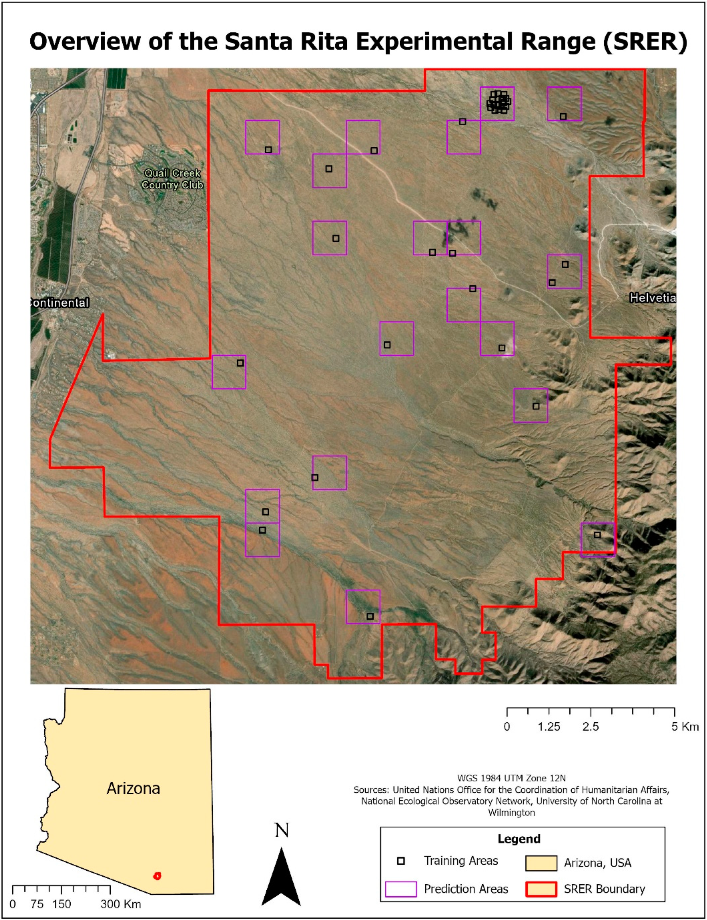
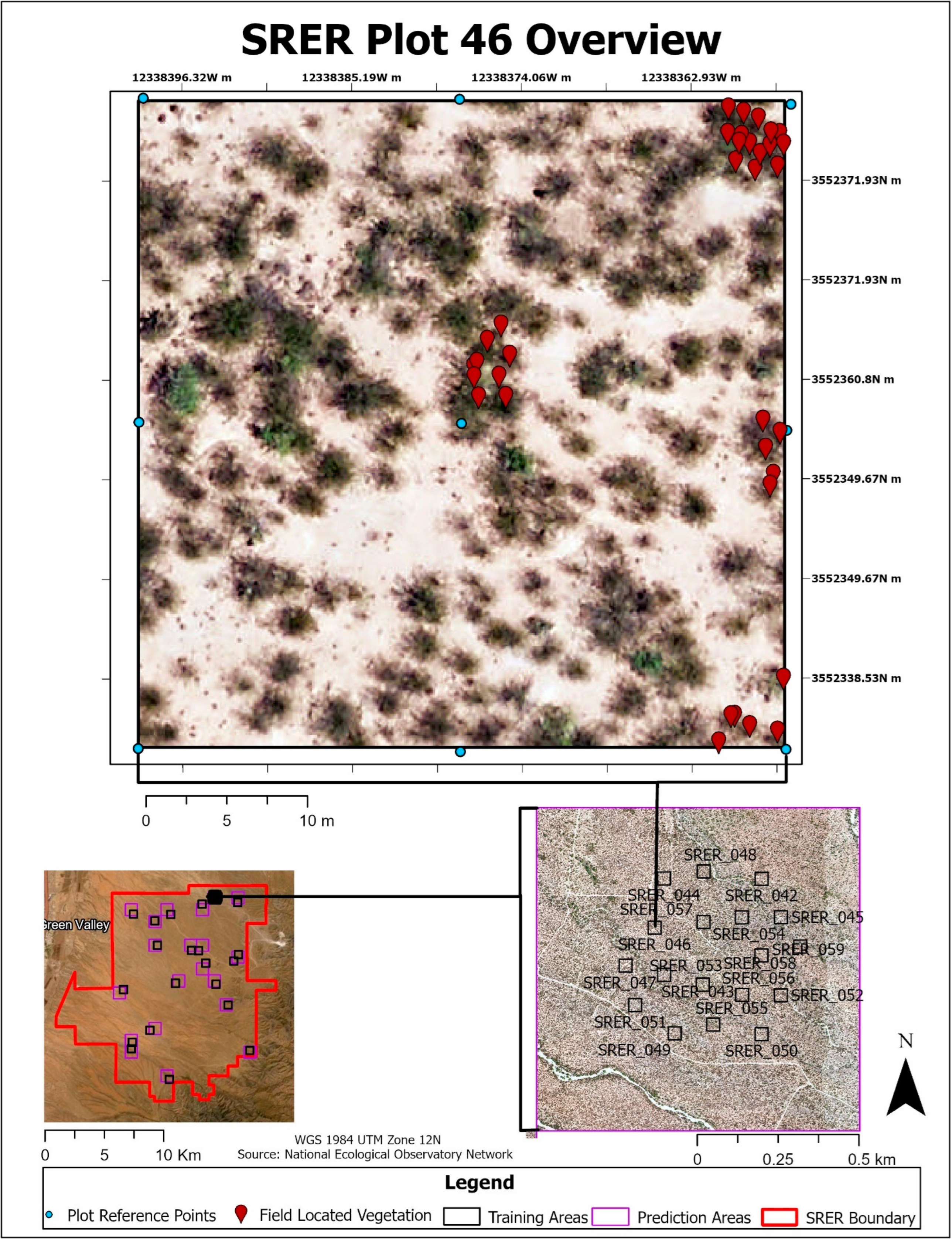
Santa Rita Experimental Range (SRER) is a NEON site that falls within Domain 14: Desert Southwest. SRER is located approximately 25 miles south of Tucson, Arizona (31.91068°N, −110.83549°W) and is one of the most extensively studied dryland regions in the United States [29]. SRER was established in 1903 by the U.S. Forest Service and managed by the U.S. Department of Agriculture until 1988, when management was handed over to the University of Arizona [29]. The initial establishment of SRER was prompted by a severe drought in the late 1800s that wiped out ranching activities in the region. At first, research activities were focused on forage plants on the range, allowing scientists to determine phenology patterns, carrying capacity, and restoration strategies for the area, with the overall goal to understand rangeland and cattle management. Over time, research focus has shifted to general studies about climate change, environmental restoration, and ecological processes [29]. SRER became a NEON study site in 2015 in pursuit of NEON’s goal to capture the ecological heterogeneity of the United States and is designated as a terrestrial core site within the network. A site overview is provided in Figure 1.

Dominant vegetation at SRER is dependent on elevation, with trees (Prosopis veluntina) and cacti (Cylindropuntia spp.) dominating elevations between 975–1100 m and shrubs (Larrea tridentata) dominating elevations below 975 m [29]. Vegetation data collected at SRER indicate that most of the site falls within the Shrub/Scrub land cover class as defined by the National Land Cover Database with FWC estimated between 30–35% and an overall mean canopy height of 2.0 m [16,29]. The Shrub/Scrub land cover class is described as areas dominated by shrubs less than five meters tall, with shrub canopy typically greater than 20% of the total vegetation [28]. Climate at SRER is characterized by semi-arid, hot conditions. Mean annual precipitation at SRER is 346 mm and occurs in a bimodal frequency, with most rainfall occurring as summer monsoons and winter rains [29]. Mean annual temperature is 19.3 °C (67 °F) with diurnal temperature swings of up to 15 °C (59 °F) regardless of season [13]. Soils at SRER are mostly composed of alluvial deposits from the nearby Santa Rita Mountains, with the most common soil subgroup being Typic Torrifluvents (hot, dry floodplain soils) [13]. Soils at higher elevations have higher organic content, less salt, and lower temperature compared to soils at lower elevations [13].

All data were downloaded from the NEON data portal (neonscience.org) and are listed and described in

Table 1. Data products downloaded from the NEON Data Portal. DP1 and DP2 indicate Level-1 and Level-2 data products, respectively.

Data Product Name	Data Format	Description
Discrete Return LiDAR Point Cloud (DP1.3003.001) [31]	LAZ	Point locations recorded in meters with spatial resolution ranging from 0.15–1.5 m
High-resolution orthorectified camera imagery (DP1.30010.001) [32]	GeoTIFF	White balanced, 8-bit RGB imagery collected at 0.1 m spatial resolution
Vegetation Indices (DP2.30026.001) [33]	GeoTIFF	Collection of five spectral indices (ARVI, EVI, NDVI, PRI, and SAVI) derived from multispectral imagery at 10 m spatial resolution
Vegetation Structure (DP1.10098.001) [34]	XLSX	Database on woody plant species, location, and measurements recorded by TOS field technicians
Flight Boundaries [30]	Shapefile	Shapefile containing AOP flight boundaries for all NEON sites
TOS Sampling Locations [27]	Shapefile	Shapefile containing TOS sampling locations. Used to delineate plot boundaries for masking and clipping.

. All data and imagery are from the year 2017, as this was the first year the AOP was flown at SRER. A total of 38 plots (18 tower, 20 distributed) at SRER had in situ vegetation data collected between 2016–2019 and all were used to create training data. Plot size ranged from 400–1600 m², with distributed plots being smaller than tower plots. LiDAR point clouds, hyperspectral imagery, and high resolution RGB imagery were collected using the NEON AOP. Data were collected at a period of peak greenness to ensure all vegetation were at maximum phenological stages.

Level-0 NEON AOP data products are raw, unprocessed data and are not used in this study. Level-1 data products are derived from Level-0 through geometric, atmospheric, and radiometric correction. Level-2 data products are derived from Level-1 through additional processing depending on the data product type. Level-2 CHMs for NEON sites are corrected so that canopy heights of less than 2.0 m are automatically set to zero. With a mean canopy height of 2.0 m at SRER, the Level-2 CHM did not capture the level of detail needed for this study. Therefore, the Level-1 classified LiDAR point clouds were used to manually generate CHMs through an open-source point cloud processing software called Cloud Compare [35]. Point clouds were initially cleaned of erroneous points using a Statistical Outlier Removal (SOR) filter [35]. Next, point clouds were visually inspected to remove any other erroneous points that may have been missed by the SOR filter. Once point clouds were cleaned, a plugin for ArcGIS Pro called LAStools was used to normalize height values for the point cloud [36]. Using the “lasheight” tool from the LAStools plugin, the lowest point in each cloud was set to zero meters and all other points were scaled accordingly. Once cleaned and height normalized, point clouds were converted into CHMs, Canopy Density Models (CDMs), and Canopy Cover Models (CCMs) using the “lascover” tool from the LASTools plugin. These three data products are hereby referred to collectively as vegetation structure models. Each vegetation structure model was parameterized to match the resolution, extent, and grid placement of the Level-2 vegetation index models (NDVI, EVI, SAVI, and ARVI).

Once all vegetation structure models had been created, the Segment Mean Shift tool in ArcGIS Pro was used to segment the high resolution orthophotos into groups of pixels with similar spectral properties. Parameters of the Segment Mean Shift tool were adjusted until pixels from individual shrub crowns were delineated from their surroundings. Next, we used the Region Group tool in ArcGIS Pro to assign unique IDs for each segmented region. The Raster to Polygon tool was then used to convert the rasterized pixel groups into polygons. This polygon layer was used to generate zonal statistics for each vegetation structure and index variable by calculating the minimum, maximum, mean, range, and median pixel value for each polygon. The resulting polygon layer had these five statistics for each of the seven variables, leading to 35 total variables (shown in

Table 2. List of variables used for this study. Five statistics for each variable were calculated (minimum, maximum, mean, range, and median pixel value for each polygon) for a total of 35 numerical predictor variables and a single response variable.

Variable	Derivation	Description
Canopy Height (CH, meters)	LiDAR Point Cloud	Distance between the ground and top of vegetation canopy
Canopy Cover (CC, %)	LiDAR Point Cloud	Percent horizontal cover occupied by canopy
Canopy Density (CD, %)	LiDAR Point Cloud	Percent vertical cover occupied by canopy
Normalized Difference Vegetation Index (NDVI)	$NDVI=\frac{NIR-RED}{NIR+RED}$	Index for extracting vegetation; based on infrared reflectance (−1.0 to 1.0)
Soil Adjusted Vegetation Index (SAVI)	$SAVI=\frac{NIR-RED}{NIR+RED+0.5}\times 1.5$	Index for extracting vegetation that accounts for soil color (−1.0 to 1.0)
Atmospherically Resistant Vegetation Index (ARVI)	$ARVI=\frac{NIR-\left[RED-\gamma \left(BLUE-RED\right)\right]}{NIR+\left[RED-\gamma \left(BLUE-RED\right)\right]}$	Index for extracting vegetation that accounts for airborne particles like dust and smoke ($\gamma$ ᵞ) (−1.0 to 1.0)
Enhanced Vegetation Index (EVI)	$EVI=2.5\times \frac{\left(NIR-R\right)}{NIR+6\left(RED\right)-7.5\left(BLUE\right)+1}$	Index for extracting vegetation; based on greenness (−1.0 to 1.0)
Vegetation Cover Class	GPS located woody plants combined with CH threshold and aerial image interpretation	Categorical response variable used to classify a record as woody, non-woody, or other

and Figure S1). Figures starting with “S” can be found at the end of this document via the link to Supplementary Materials.

Once the polygon layer had been populated with data, we proceeded with polygon classification. Two classification schemes were used in this study to classify polygons: binary and multiclass. Initial classification was performed using a simple canopy height threshold like those used in other studies [2,15]. Polygons with mean canopy height values greater than or equal to ten centimeters were deemed woody and polygons with mean canopy height values less than ten centimeters were deemed non-woody. A combination of in situ vegetation location data and aerial image confirmation were then used to manually reclassify any mistakes incurred by the initial thresholding. The multiclass dataset was derived from the binary dataset, but with a new “other” class. The “other” class was used to classify polygons with mixed cover and bare ground.

Once all polygons were classified, the dataset was exported to a Comma Separated Value (CSV) file and imported into the Jupyter Notebook programming environment for Python. Initial exploratory data analysis (EDA) was performed to explore our binary and multiclass training datasets, their properties, and relationships between variables. In the process of generating zonal statistics, some polygons did not cross the centroid of a single pixel, resulting in 151 records with null values. Our initial data cleaning removed these null records, leaving us with a total of 4339 polygons across the 38 training plots. Under the binary classification scheme, the woody and non-woody classes each comprised about half of the polygons (51.9%, 48.1%, respectively). Under the multiclass scheme, the woody class was more abundant (50.1%), followed by non-woody (37.6%), then other (12.3%).

Variable correlation was assessed with heat maps to understand the relationships between each variable. High correlation was observed between certain statistics for the same variable (e.g., mean and max, max and range) which is expected due to the nature of such statistics. High correlation was observed between the statistics for the canopy cover and canopy density variables, which is thought to be due to the growth form of shrubs (somewhat cube-like or spherical). High correlations were also observed between all vegetation indices due to their shared property of having higher values for photosynthetically active vegetation and lower values for anything else. All variables were also right skewed, with the most skewness observed in the canopy height statistics. This indicates that high values for any given vegetation index or structure variable–indicative of vegetation–are relatively uncommon in the training dataset and more field collection may be necessary to bolster the representation of woody plant properties in the data.

After EDA, each dataset was input into each machine learning model and performance was assessed. Five-Fold Cross Validation (FFCV) was used to train each model and assess its predictions. Performance was compared between decision tree-based and non-decision tree-based models for initial model selection. The top variables were then ranked by importance from all selected models using a simple voting method, where if a variable was in the top ten for a given model, it received one vote. Ten was chosen as the cutoff due to importance rapidly decreasing after the top ten variables for most models. The Boruta package in Python (Python Version 3.9.8, Python Software Foundation, Wilmington, DE, USA) was then used to further supplement and verify the initial variable selection method [37]. The Boruta package allowed us to see variable importance for each of the five folds on the FFCV, granting more insight into variable importance.

Once top variables had been selected, models were reassessed using FFCV. Next, we performed model tuning by making adjustments to each model’s hyperparameters using a Grid Search method to determine the ideal settings for each model [38]. A list of all settings tested for each model can be found in

Table 3. Hyperparameter settings tested with the Grid Search Method. Models include Decision Tree (DT), Bagging (BAG), Random Forest (RF), Gradient Boost (GB), eXtreme Gradient Boost (XGB), Light Gradient Boost (LGB), Ada Boost (ADA), and Cat Boost (CAT).

Hyperparameter	Values Tested	DT	BAG	RF	GB	XGB	LGB	ADA	CAT
Number of Trees	10, 100, 1000	X *	X	X	X	X	X	X	X
Max Tree Depth	1, 5, 10	-	X	X	X	X	X	- *	X
Max Number of Leaf Nodes	None, 5, 10	-	X	X	X	X	-	-	-
CCP Alpha	0.0, 0.1, 0.3, 0.5	-	X	X	X	X	-	-	-
Learning Rate	0.001, 0.01, 0.1	-	-	-	X	X	X	X	X
Subsample	0.5, 0.7, 1.0	-	-	-	X	X	X	-	X
Loss Function	deviance, exponential	-	-	-	X	-	-	-	-
Split Function	Friedman MSE, Squared Error	-	-	-	X	-	-	-	-
Number of Covariates Considered per Split	$\sqrt[2]{\# of variables}$; ${\log }_2(\# of variables)$	-	-	X	X	X	-	-	-
Number of Leaves	10, 20, 30, 40	-	-	-	-	-	X	-	-
Minimum Child Samples	10, 15, 20, 25	-	-	-	-	-	X	-	X

* An ‘X’ indicates that the hyperparameter was tested and a ‘-’ indicates that the hyperparameter was not applicable.

and visualized at plot level in Figure S1.

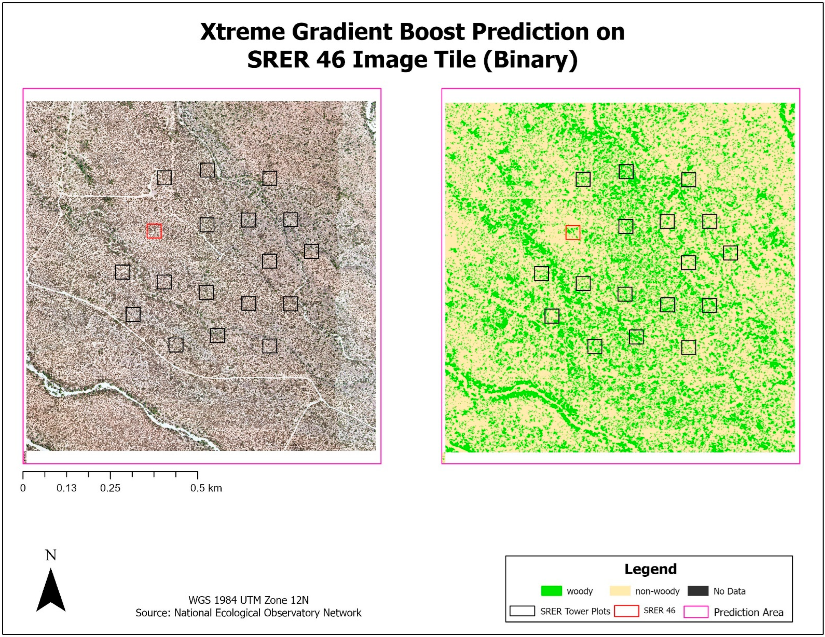
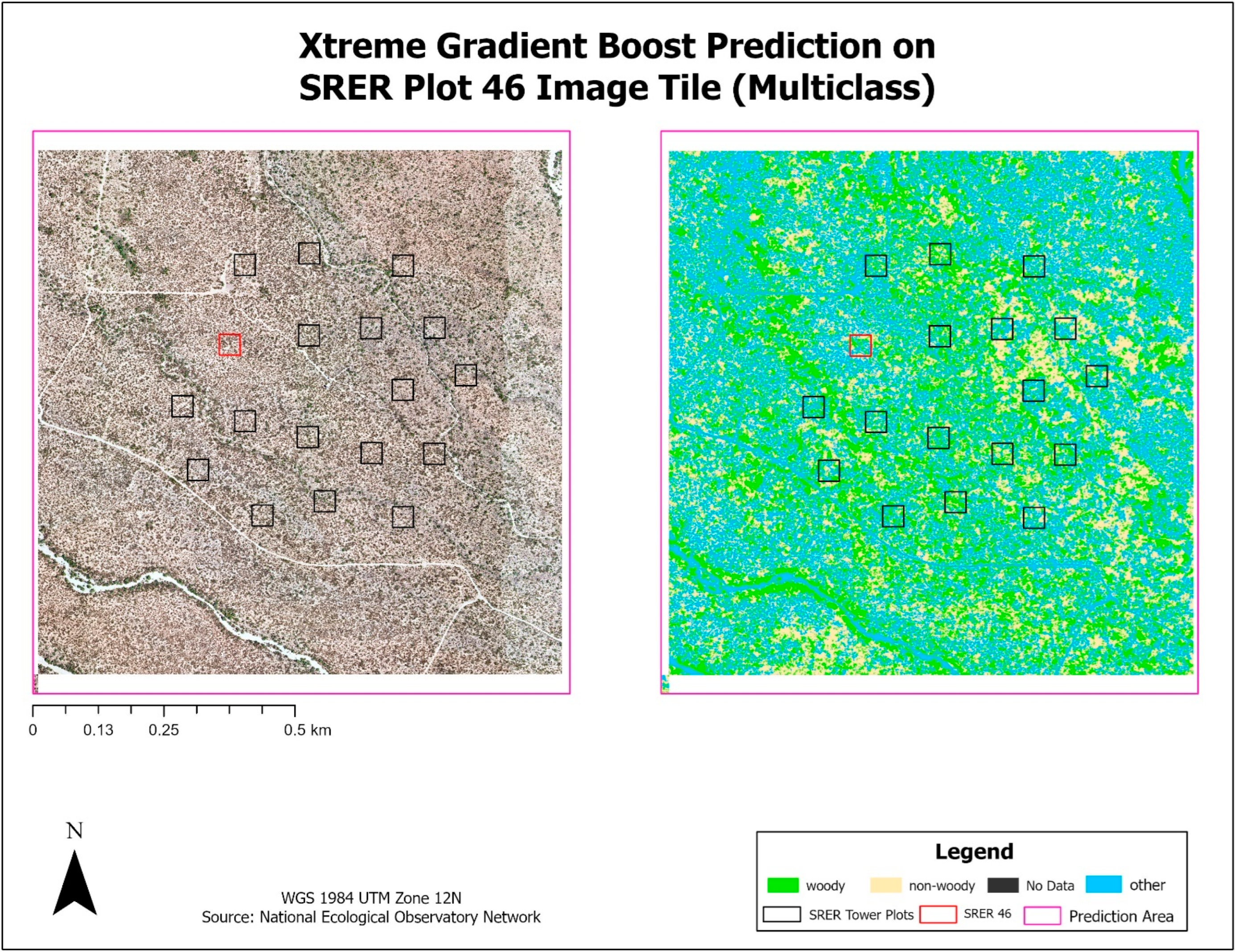
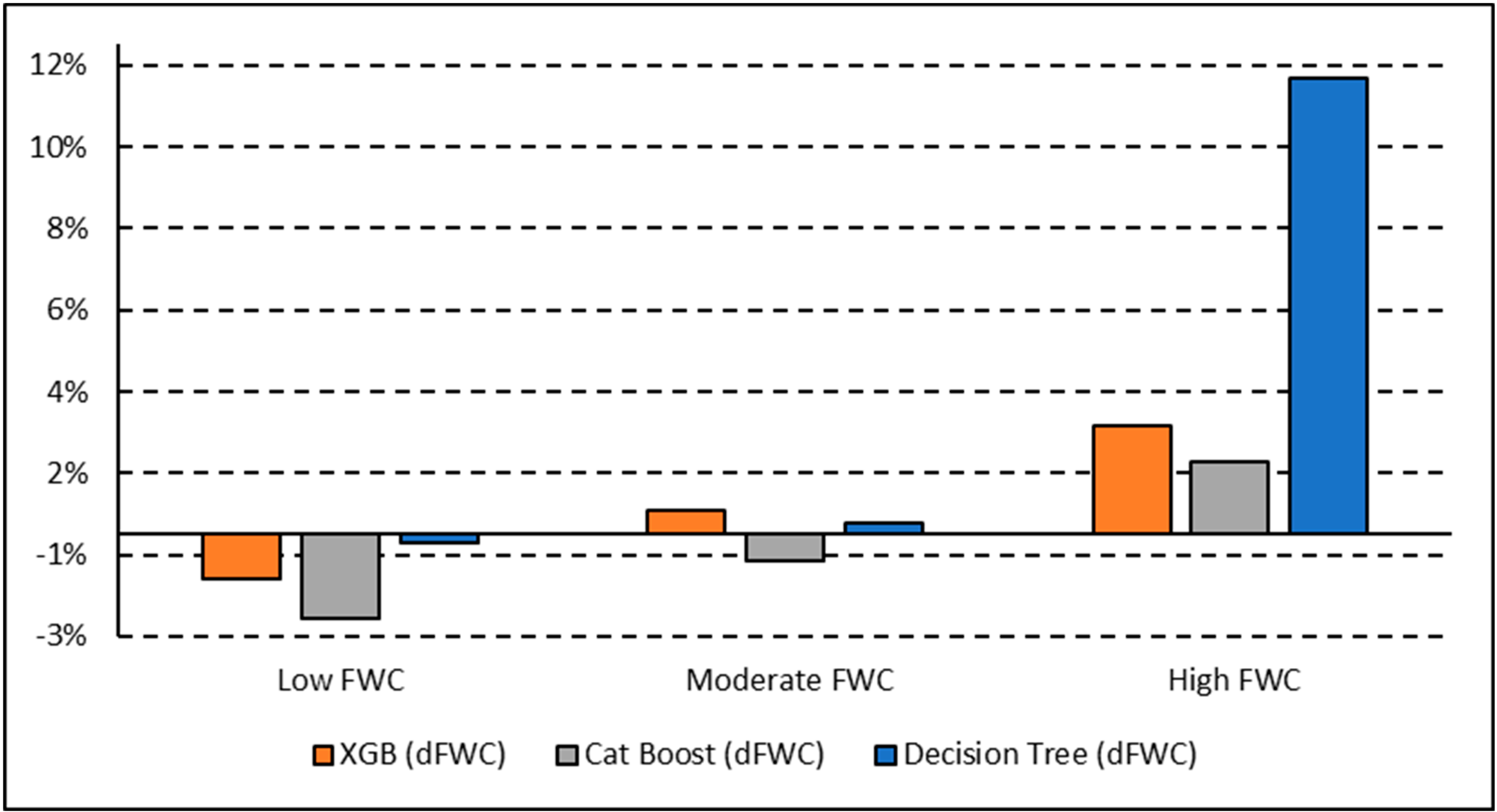
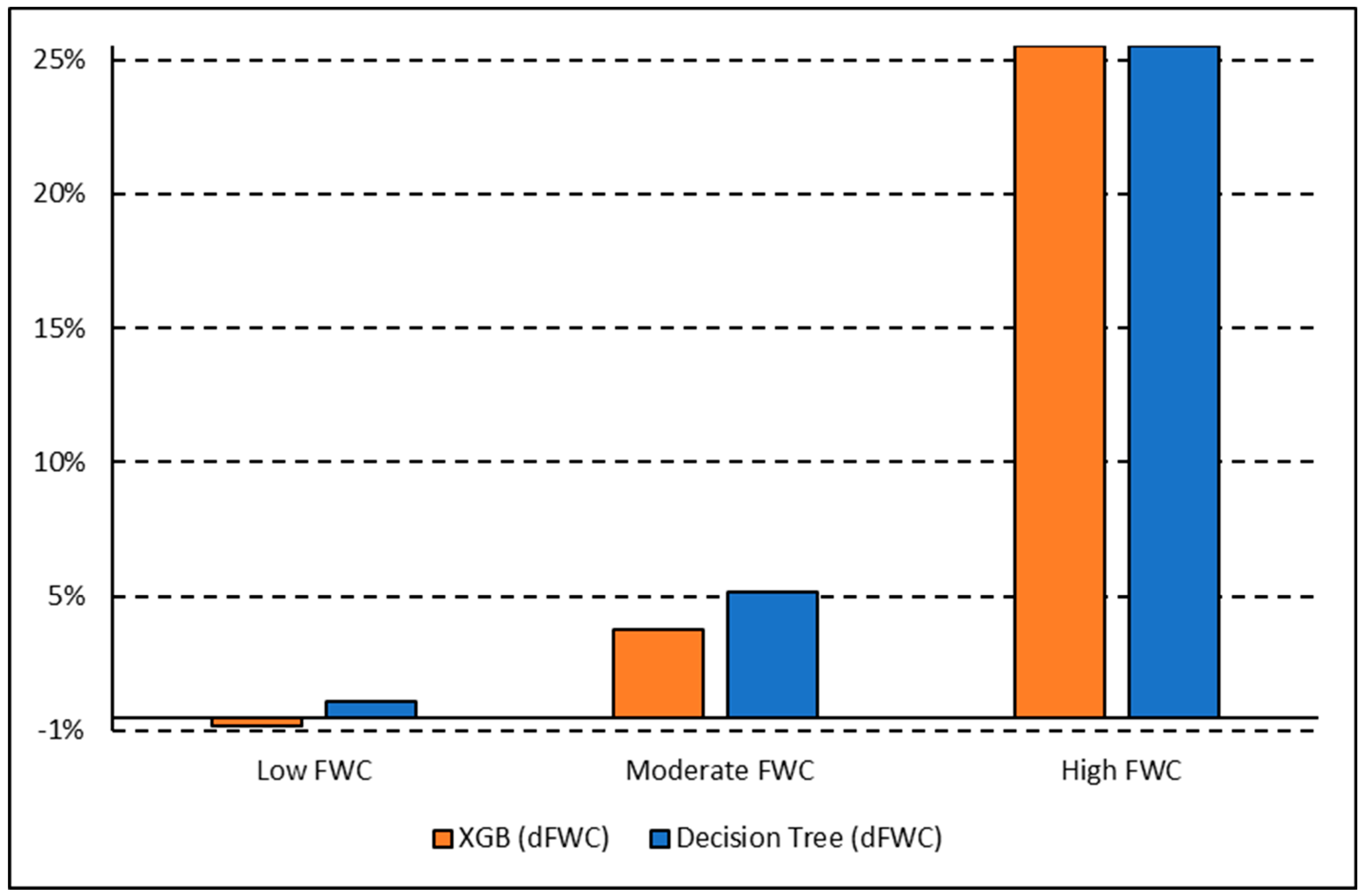
Once tuned, the finalized models predicted woody plant cover for the 1.0 km² image tile that each training plot was contained within. A total of 20 image tiles were predicted due to the 18 tower plots all falling within a single image tile and another case where two plots fell within the same image tile. The results from each model were exported as a CSV and brought into ArcGIS Pro, where they were joined back to a corresponding polygon layer. A prediction field for each model and classification scheme was calculated from the model output, resulting in a polygon layer with predictions from each model. FWC was calculated from the training data and compared to predicted FWC for each model by calculating the difference in FWC (dFWC). Training sites were also ranked by FWC into Low, Moderate, and High to assess if canopy density influenced dFWC.

3. Results

3.1. Model Selection

The goal for initial model selection was to determine the best possible polygon classification models, as higher polygon classification accuracy was assumed to yield higher accuracy of FWC estimates. Intermediate results from model selection for each classification scheme are reported in Figures S2–S5. Results for the multiclass classification scheme do not include the Cat Boost model, as it was not supported with the same methodology used for the other models. Runtimes for each initial model can be found in Figures S6 and S7.

Initial classification models agreed that decision tree-based models have higher classification performance metrics and prediction stability, but longer runtimes compared to non-decision tree-based models. Most models had higher specificity than sensitivity, indicating that the non-woody classes were being classified with higher accuracy than the woody class. Multiclass models took longer to run in general compared to binary models and overpredicted the ‘other’ class, leading to much higher specificity than sensitivity. This overprediction is thought to be due to the inclusion of mixed-cover polygons in the ‘other’ class, giving it properties of both the ‘woody’ and ‘non-woody’ class in some cases.

In general, non-decision tree-based models underperformed the decision-tree based models. While the logistic regression model appears to perform well at first glance, it was unable to run with all variables in the dataset upon initial model selection due to unexpected errors with the LogisticRegression package in Python. All non-decision tree-based models were ruled out through our model selection process and were not considered in the next steps.

3.2. Variable Selection & Model Tuning

Variable selection was initially performed using the top ten variables from all binary models. Binary models were chosen for variable selection as they had higher performance than multiclass. The results from the first variable selection are shown in Table S1. After initial variable selection, the Boruta package in Python was used to assess variable importance. Agreement between the Boruta method and initial voting method was assessed to add and remove variables. Final variable selection is listed in

Table 4. Final variable selection after the Boruta method. Variables with more than three ‘keep’ votes from Boruta were added to the list and variables with more than three ‘reject’ votes were removed from the list.

Variable	Number of Votes
EVI (median)	6
ARVI (mean)	6
SAVI (median)	5
Canopy Height (mean)	5
ARVI (median)	5
EVI (mean)	5
NDVI (max)	5
NDVI (mean)	5
SAVI (mean)	5
SAVI (max)	4
ARVI (max)	4
NDVI (median)	3
EVI (max)	3

.

After both rounds of variable selection, we had determined that 13 of the 35 variables were of high importance and were the only variables considered when moving forward with model tuning and estimating FWC. Final selected variables include the mean, median, and maximum statistics for all vegetation indices and mean Canopy Height. Intermediate results following variable selection are shown in Figures S8–S13. Compared to the initial models, the variable-selected model accuracy decreased from 67.8–69.8% to 67.0–69.5% for the binary scheme and from 59.2–61.1% to 57.9–60.8% for the multiclass scheme.

Overall, variable selection resulted in a slight decrease in model accuracy and stability across all models, likely due to there being less information for models to make predictions from. Next, model tuning was performed with the Grid Search method to determine the best hyperparameters for each model and attempt to regain some of the lost accuracy. Results from the binary Grid Search are listed in

Table 5. Optimal hyperparameters for each binary model after variable selection as determined by grid search.

Hyperparameter	DT	BAG	RF	GB	XGB	LGB	ADA	CAT
Number of Trees	1	100	1000	100	1000	1000	1000	100
Max Tree Depth	-	10	5	5	5	10	-	10
Max Number of Leaf Nodes	-	None	None	None	None	-	-	-
CCP Alpha	-	0.0	0.0	0.0	0.0	-	-	-
Learning Rate	-	-	-	0.01	0.001	0.001	0.01	0.1
Subsample	-	-	-	0.5	0.5	0.5	-	0.7
Loss Function	-	-	-	deviance	-	-	-	-
Split Function	-	-	-	Squared error	-	-	-	-
Number of Covariates Considered per Split	-	-	auto	log2	auto	-	-	-
Number of Leaves	-	-	-	-	-	10	-	-
Minimum Child Samples	-	-	-	-	-	15	-	10

and results from the multiclass grid search are listed in Table S2 in Supplementary Materials.

Each model was run with FFCV after tuning to assess final model performance, with binary model results shown in Figure 2 and Figure 3 and multiclass model results shown in Figures S14 and S15. Final model runtimes can be found in Figures S16 and S17 in Supplementary Materials.

Changes to model accuracy, standard error, sensitivity, and specificity between each binary model refinement step are presented in

Table 6. Binary model performance metrics between each refinement step.

	Overall Accuracy			Standard Error			Sensitivity			Specificity
Model	Initial	Variable Selection	Final	Initial	Variable Selection	Final	Initial	Variable Selection	Final	Initial	Variable Selection	Final
DT	67.8%	68.3%	68.3%	0.8%	1.7%	1.7%	66.0%	68.0%	68.0%	70.0%	69.0%	69.0%
BAG	67.9%	67.0%	69.0%	9.1%	0.9%	0.7%	67.0%	65.0%	67.0%	69.0%	69.0%	71.0%
RF	68.0%	66.8%	69.4%	1.1%	1.1%	1.4%	69.0%	65.0%	68.0%	71.0%	69.0%	71.0%
GB	69.8%	69.3%	69.2%	0.1%	1.1%	1.1%	68.0%	67.0%	69.0%	72.0%	71.0%	70.0%
XGB	69.6%	69.2%	69.3%	1.0%	1.8%	1.1%	68.0%	67.0%	67.0%	72.0%	72.0%	72.0%
LGB	69.6%	69.1%	68.9%	14.7%	0.9%	1.4%	69.0%	66.0%	67.0%	68.0%	72.0%	71.0%
ADA	68.8%	68.3%	68.2%	1.2%	1.2%	1.3%	68.0%	68.0%	68.0%	71.0%	68.0%	68.0%
CAT	69.6%	69.5%	69.3%	0.8%	1.2%	0.9%	66.0%	67.0%	67.0%	70.0%	72.0%	72.0%

. Compared to initial model runs, variable selection caused slight decreases to overall accuracy (max decrease was 1.2% for Random Forest). This is expected, as over half of the initial variables were removed from the training dataset. Variable reduction also reduced the large standard errors observed in the Bagging and Light Gradient Boost models. Final model accuracy improved from initial models for all independent models (Decision Tree, Bagging, and Random Forest) and declined for all sequential models. Given that all final model accuracies are within 1–2% of initial models and standard errors are also ~1–2%, we can generally conclude that final models perform nearly as accurately as initial models, but at faster setup and runtimes now that optimal variables and hyperparameters have been determined. A corresponding table for multiclass can be found in Table S3.

3.3. FWC Estimates

After the models had been refined and finalized, they were used to predict the 1 km² image tiles to demonstrate how these models can predict woody vegetation and estimate FWC in areas beyond the training sites with no in-situ data. FWC estimates from the training data were used to categorize each plot into low, moderate, or high FWC. The plots with minimum (Plot 14), median (Plot 46), and maximum (Plot 19) FWC were used to map the top two model predictions (XGB and Cat Boost) and the worst model prediction (DT) with respect to dFWC. The XGB model had the smallest dFWC (Figure 4) and was used to map image tile predictions. Plot 46 maps are shown in the following map series (Figure 5, Figure 6, Figure 7, Figure 8, Figure 9 and Figure 10). Maps for Plots 14 and 19 are included in Figures S18–S29. Image segmentation on training plots was initially performed at the extent of each training plot. Subsequent image segmentation for predicting image tiles was performed at the extent of the image tile, so predicted training plots have slight differences in the number, size, and shape of polygons, but these differences are generally subtle and are not expected to have dramatic impacts on FWC estimations.

3.3.1. SRER Plot 46: Moderate FWC

Overall, Plot 46 had high agreeance in FWC between the training and prediction classification methods (mean dFWC for XGB = 1.93%). The XGB model slightly overpredicted woody vegetation overall, as indicated by the positive dFWC value and visual inspection showing clustered predictions in areas of woody vegetation. This clustering behavior overlooks canopy gaps that manual annotation can discern. The prediction tiles for this plot highlights areas of woody vegetation consistently between classification schemes (dFWC between schemes = 1.5%). The multiclass scheme shows additional detail with the non-woody class potentially highlighting areas of interest for further field data collection and verification.

3.3.2. Plot Complexity Analysis

dFWC was broken down between each of the FWC classes to assess if FWC was related to dFWC. Plots were sorted into classes by FWC, with the highest, middle, and lowest thirds falling into high, moderate, and low FWC, respectively. The results are graphed in Figure 11 and Figure 12. The overall trend shows that plots with high FWC had higher dFWC, regardless of classification scheme.

4. Discussion

Overall, we have answered all three of our RQs with the following conclusions:

RQ1: 

What classification models and schemes most accurately classify woody vegetation at a dryland NEON site with low canopy complexity?

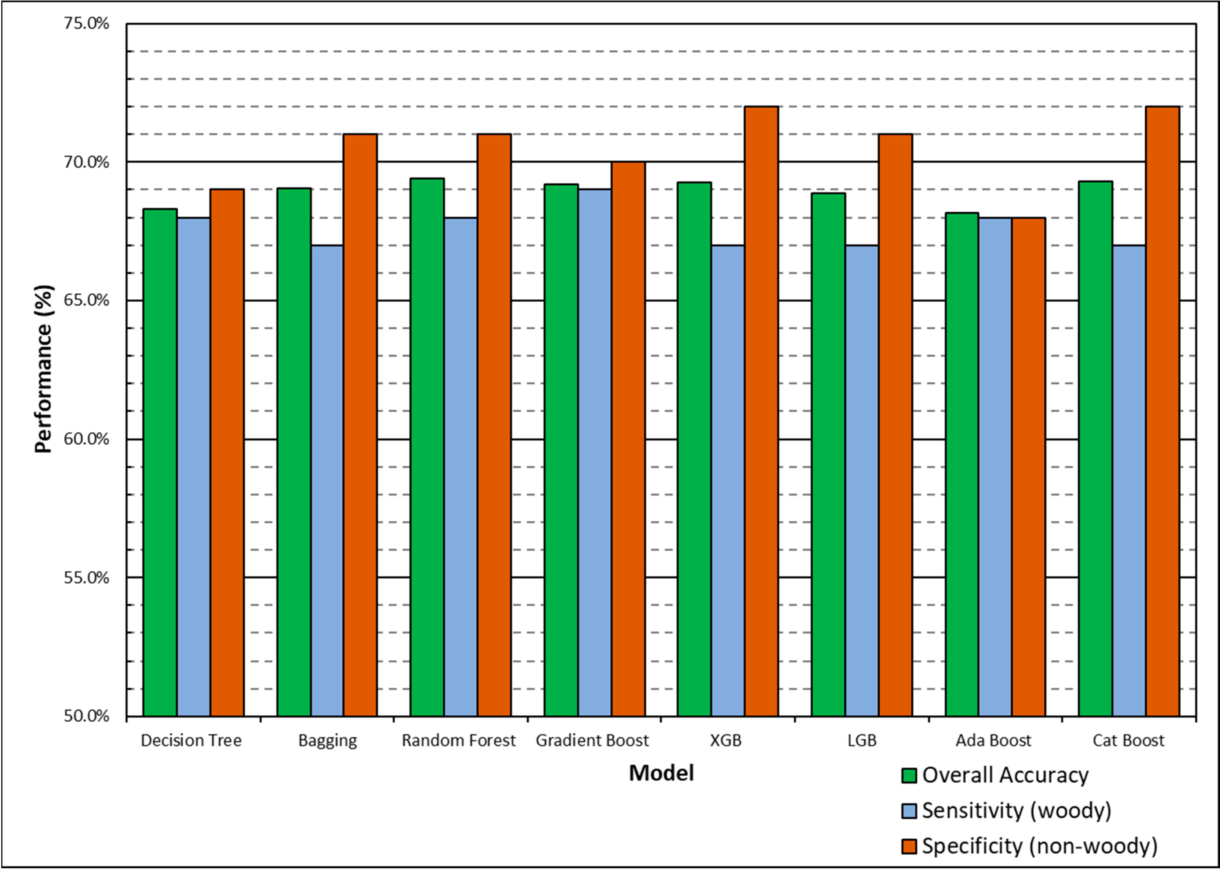
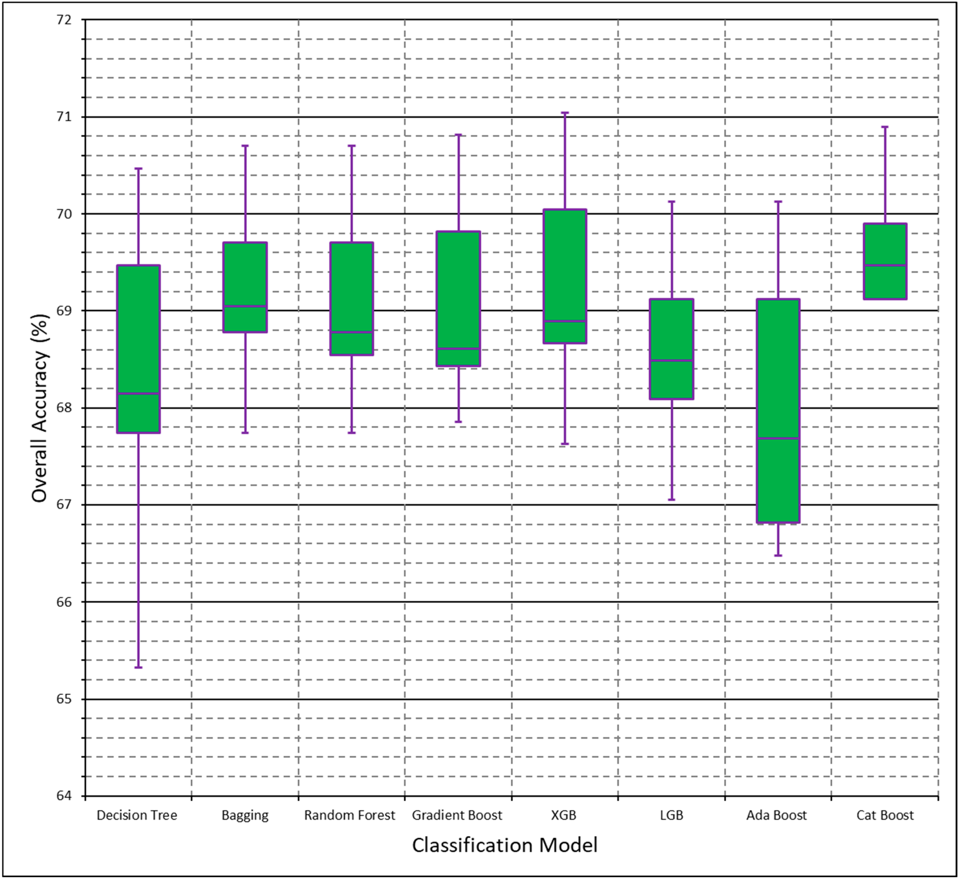
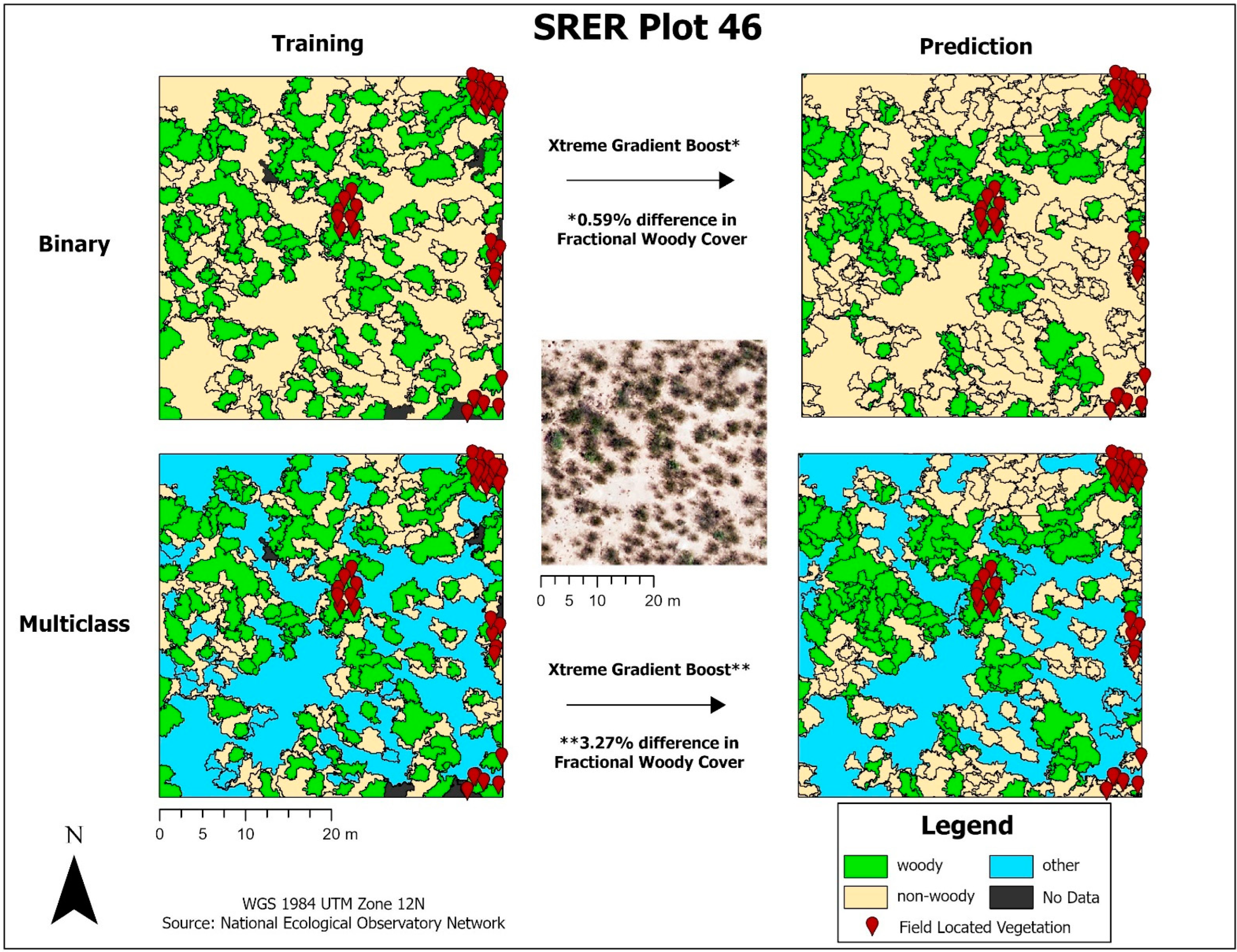
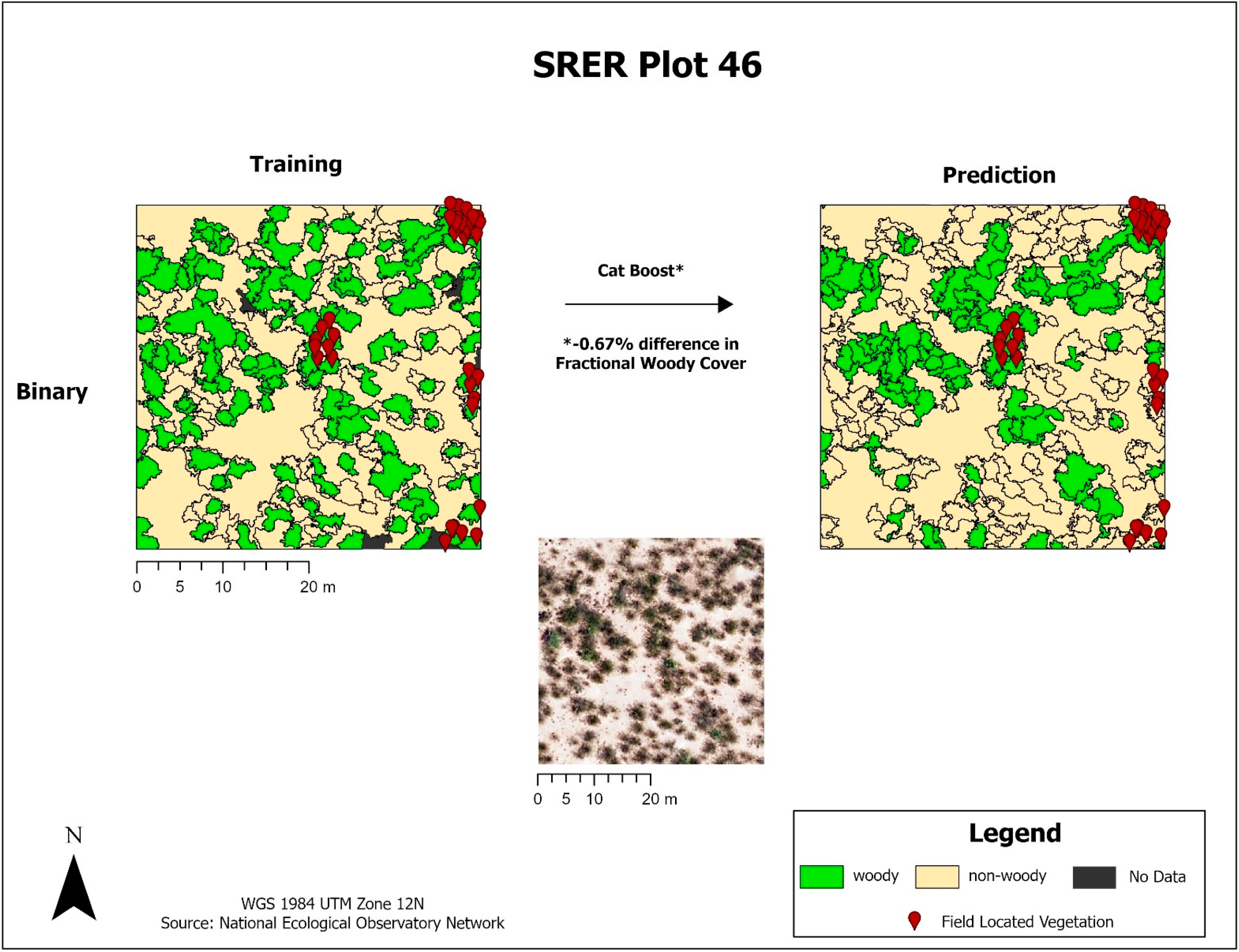
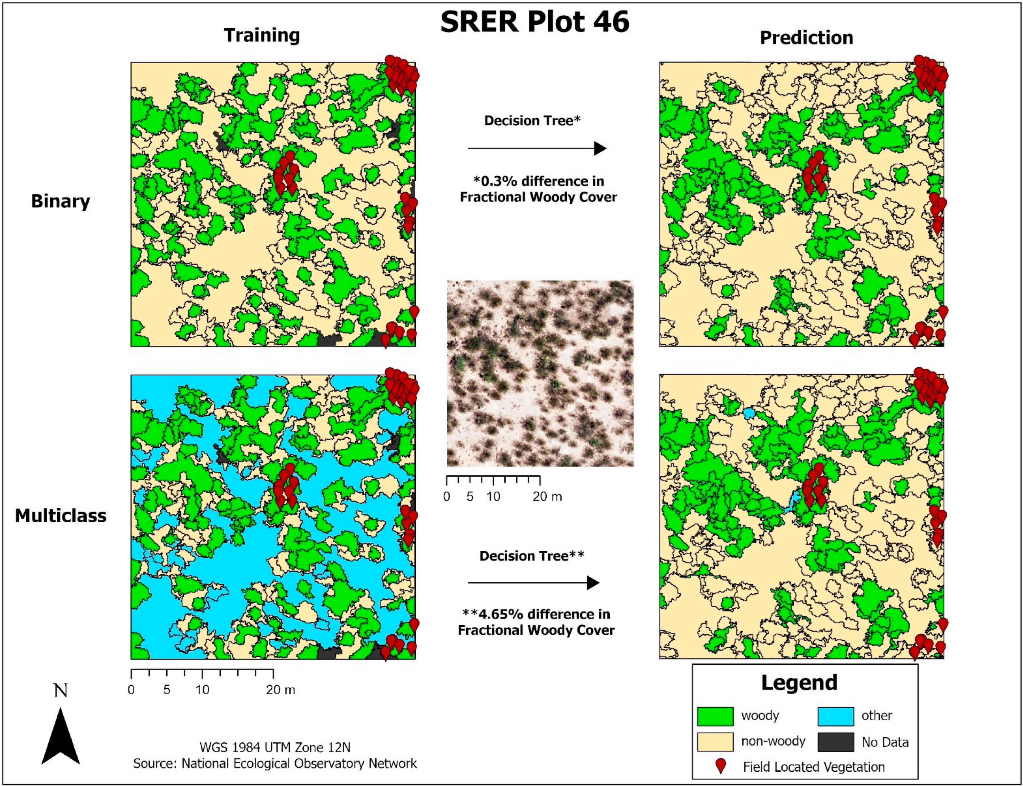
Decision tree-based models had higher model performance compared to non-decision tree-based models, with Gradient Boost having higher polygon-based classification accuracy in both initial and finalized models. We have also identified limitations with scikit-learn models, as Logistic Regression could not run without the removal of variables and Cat Boost could not be implemented with the multiclass dataset. In this study, we test both a binary (‘woody’ vs. ‘non-woody’ cover) and multiclass (‘woody’ vs. ‘non-woody’ vs. ‘other’ cover) scheme. It is important to denote that the ‘non-woody’ class in the binary scheme does not solely represent vegetation cover, as the ‘non-woody’ class can also represent non-vegetated areas such as roads, water, and bare ground. Conversely, the ‘non-woody’ class in the multiclass scheme solely represents vegetation cover, with the ‘other’ class handling non-vegetated cover like roads, water, and bare ground. The binary classification scheme had higher overall accuracy compared to multiclass, but the multiclass scheme may provide additional feature delineation that the binary scheme does not provide. More field data is needed to assess the type of features that the non-woody class represents, if there are common features. Narrowing down the high performing models and classification scheme uses will save time for future research by ruling out underperforming models and demonstrating the advantages of different classification schemes.

RQ2: 

What variables are most important for classifying woody vegetation at a dryland NEON site with low canopy complexity?

The only high-importance vegetation structure variable was mean canopy height, and all vegetation indices were deemed highly important, but only their mean, median, and maximum statistics. Narrowing down the best variables for classifying woody vegetation will save time for variable collection and processing in future work. For example, the generation of canopy cover and canopy density variables was unnecessary for this study. Model runtimes and error also improve with a smaller number of highly important variables. The variables tested in this study are only a small handful of the wide variety of variables collected by NEON, and future studies might consider testing variables such as leaf area index and canopy moisture content.

RQ3: 

How do FWC estimates derived from manual classification methods compare to FWC estimates derived from ML models?

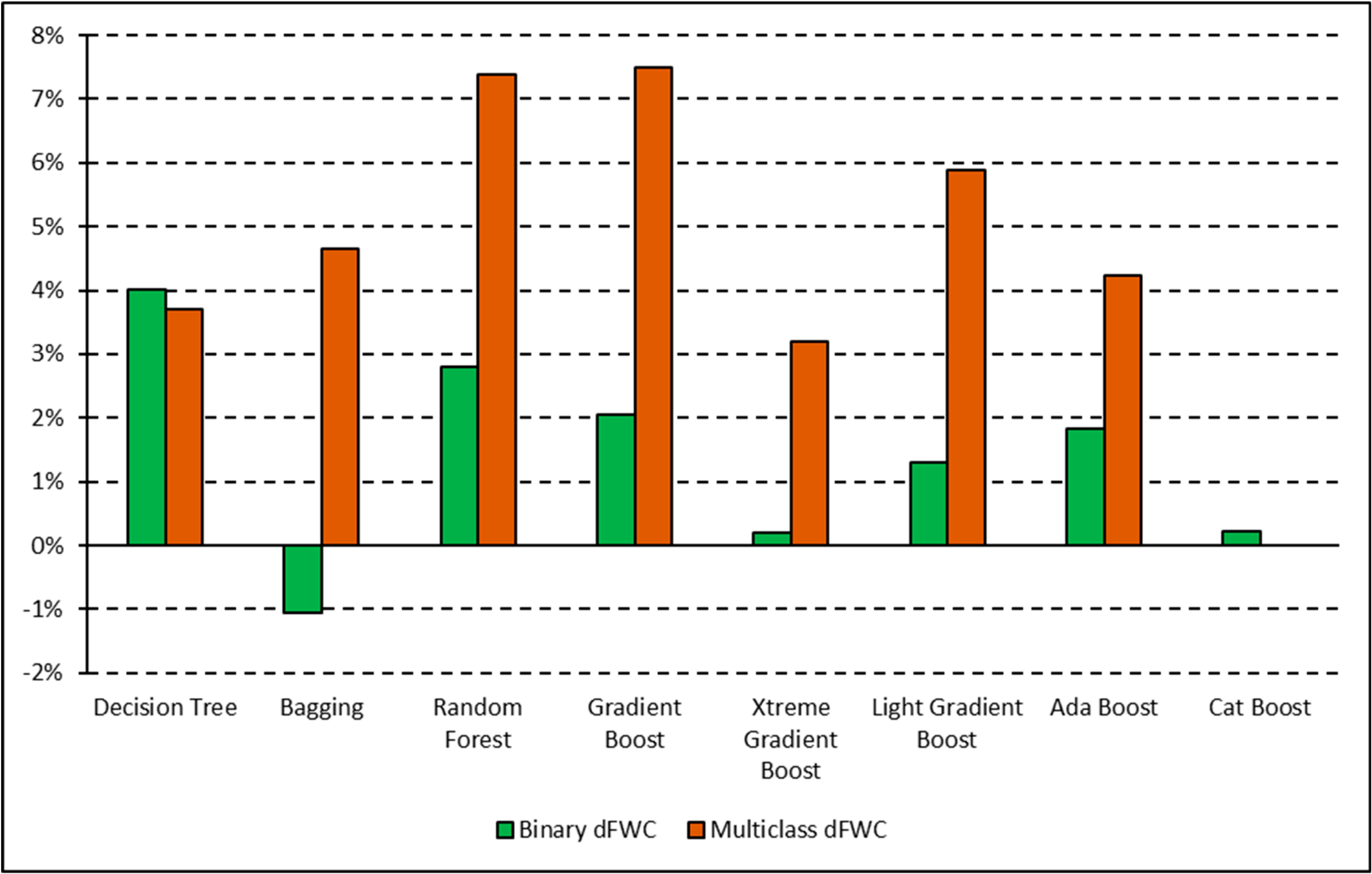
The XGB model had the lowest overall dFWC (0.2% for binary, 3.2% for multiclass) when compared to the manually annotated training data, indicating that it predicted gross FWC estimations with the highest agreeance. This dFWC metric has not been spatially assessed, however, to determine spatial accuracy. dFWC also differed depending on FWC at the plot level, with high FWC plots having much higher dFWC across models. This indicates that these models may perform best in low to moderate FWC areas, which is where most of the training data has been collected. More field sampling in the southern portions of SRER, where vegetation density and complexity is more robust, may improve estimates in areas of high FWC, but also introduce more prediction error for the low and moderate classes. Overall, manual classification methods have estimated FWC at 34.8% across all training plots, with a dFWC range from −1.1–7.5% when considering all models. This mostly falls within the 30–35% range suggested by [16], indicating that both manual and automated classification methods are reasonably accurate overall.

While this study provides a good starting point for estimating FWC in a semi-arid region, it only provides a snapshot in time of the dynamic WPE process. As time progresses and WPE occurs, the annual data collected by NEON will be crucial for time-series analysis and change detection to assess the true extent and rate of WPE at SRER. With this study serving as a baseline establishment of FWC estimation methods, further studies that replicate these methods can be used with subsequent years of in situ and remote sensing data collection to monitor WPE throughout the study area and possibly throughout other similar areas of interest.

We also recognize that the variables used in this study are by no means a comprehensive representation of those that can be collected or derived to fully describe woody vegetation, nor do they represent all potential vegetation variables collected by NEON. Further variable selection is therefore necessary to assess variables like Leaf Area Index (LAI), Ecohydrological Index (EI), and Soil Moisture Index (SMI), to name a few. Finally, we also recognize that the training data used in this study is small relative to other studies. With the goal of using solely NEON data for this study, we were limited to the amount of training data included by the amount of data collected at the time of this study. Using data from other similar NEON sites, such as the San Joaquin Experimental Range (SJER), or future in situ and remote sensing data collected at SRER, would be expected to improve classification results.

5. Conclusions

The results from this study lay the groundwork for future use and implementation of NEON data by determining the best models, variables, and hyperparameter settings for predicting woody plant cover at SRER along with exploring different classification schemes. Land managers at SRER can apply these ML models to develop and monitor woody plant management strategies within their domain. With a planned mission time of 30 years, the volume of data collected at SRER will continue to grow, allowing developed models to be augmented and reassessed as land cover change occurs. This study also demonstrates the capabilities of using solely open-source NEON data and open-source code to train prediction models without any additional data collection—a workflow that can be implemented for any NEON site from anywhere in the world.

Land managers in other dryland landscapes where WPE is occurring can also use the methods from this study as a framework for developing their own models, and possibly use the models trained in this study to predict woody cover within their own domain, provided the same data are available and the sites have similar vegetation structure and distribution patterns. A prime example of such a location is the San Joaquin Experimental Range (SJER), which is the only other study area within the Desert Southwest Domain (D14) established by NEON. Using the models from this study to assess model performance at other manually classified training plots would provide more insight into model performance outside of their own training data.

With NEON in its infancy, limited work has been published that relies solely on its data to delineate or classify woody vegetation. Two other studies, 22,23], have accomplished this, but their chosen NEON sites were representative of open and closed woodland ecosystems, respectively. This study fills a research gap by developing woody plant detection models in shrub/scrub ecosystems with relatively low vegetation complexity. As suggested by [23], the prediction models used for this study had higher classification accuracy than those conducted in more complex ecosystems, supporting their suggestion. The classification methods for this study are simpler however, as we only tested very general classes, rather than classifying at species level. The simplification of both the modeling framework and the vegetation complexity may be working in tandem to drive classification accuracy higher. Dryland regions have been traditionally defined by an aridity index (AI) as described in our introduction by the ratio P/PET [1]. Use of ML to model dryland migration under the context of climate change has consistently predicted an overall expansion of global dryland cover [1]. In 2021, Berg & McColl [39] suggested that a new index, coined the ecohydrological index (EI), may be more appropriate for predicting dryland migration, as it takes plant physiology and soil moisture into account rather than solely relying on climatic variables. In their study, Berg & McColl [39] found that dryland expansion will not occur under the RCP 8.5 climate scenario when using EI as a metric, which is highly contradictory to past studies. Therefore, further investigation of EI as a predictor of drylands is necessary both under the current and future climate models published by the IPCC. Luckily, all variables needed to calculate EI are collected and publicly available through the NEON data portal, further highlighting its future role in investigating ecosystem dynamics.

The National Ecological Observatory Network (NEON) is the largest and most comprehensive ecological dataset of its kind, with the promise of 30 continuous years of high-resolution remote sensing and in situ monitoring over its 81 field sites. Discovering how we can use solely NEON data to train Machine Learning (ML) and Artificial Intelligence (AI) models for land cover prediction is vital to land managers throughout the world looking for new and cost-effective ways to gain insight to their changing landscapes. As more data is collected at these NEON sites, models and methods such as those tested in this study have the potential to evolve in ways that will inform land management strategies far into the future. Successive studies conducted with this data may investigate other ML/AI models, additional variables collected by NEON, and change detection of FWC over time and in response to woody plant management regimes.

References

1. Feng, S.; Fu, Q. Expansion of Global Drylands under a Warming Climate. Atmos. Chem. Phys. 2013, 13, 10081–10094. [Google Scholar] [CrossRef] [Green Version]
2. Gaughan, A.E.; Kolarik, N.E.; Stevens, F.R.; Pricope, N.G.; Cassidy, L.; Salerno, J.; Bailey, K.M.; Drake, M.; Woodward, K.; Hartter, J. Using Very-High-Resolution Multispectral Classification to Estimate Savanna Fractional Vegetation Components. Remote Sens. 2022, 14, 551. [Google Scholar] [CrossRef]
3. Shukla, P.R.; Skea, J.; Calvo Buendia, E.; Masson-Delmotte, V.; Pörtner, H.-O.; Roberts, D.C.; Zhai, P.; Slade, R.; Connors, S.; van Diemen, R.; et al. Climate Change and Land: An IPCC Special Report on Climate Change, Desertification, Land Degradation, Sustainable Land Management, Food Security, and Greenhouse Gas Fluxes in Terrestrial Ecosystems; Intergovernmental Panel on Climate Change: Geneva, Switzerland, 2019; pp. 1–874. [Google Scholar]
4. Archer, S.R.; Andersen, E.M.; Predick, K.I.; Schwinning, S.; Steidl, R.J.; Woods, S.R. Woody Plant Encroachment: Causes and Consequences. In Rangeland Systems; Briske, D.D., Ed.; Springer Series on Environmental Management; Springer International Publishing: Cham, Switzerland, 2017; pp. 25–84. ISBN 978-3-319-46707-8. [Google Scholar]
5. Podwojewski, P.; Grellier, S.; Mthimkhulu, S.; Titshall, L. How Tree Encroachment and Soil Properties Affect Soil Aggregate Stability in an Eroded Grassland in South Africa. Soil Sci. Soc. Am. J. 2014, 78, 1753–1764. [Google Scholar] [CrossRef]
6. Sala, O.E.; Maestre, F.T. Grass-Woodland Transitions: Determinants and Consequences for Ecosystem Functioning and Provisioning of Services. J. Ecol. 2014, 102, 1357–1362. [Google Scholar] [CrossRef]
7. Venter, Z.S.; Cramer, M.D.; Hawkins, H.-J. Drivers of Woody Plant Encroachment over Africa. Nat. Commun. 2018, 9, 2272. [Google Scholar] [CrossRef] [Green Version]
8. Faber-Langendoen, D.; Keeler-Wolf, T.; Meidinger, D.; Josse, C.; Weakley, A.; Tart, D.; Navarro, G.; Hoagland, B.; Ponomarenko, S.; Fults, G.; et al. Classification and Description of World Formation Types; U.S. Department of Agriculture, Forest Service, Rocky Mountain Research Station: Ft. Collins, CO, USA, 2016; p. RMRS-GTR-346. [Google Scholar]
9. de Jong, R.; de Bruin, S.; de Wit, A.; Schaepman, M.E.; Dent, D.L. Analysis of Monotonic Greening and Browning Trends from Global NDVI Time-Series. Remote Sens. Environ. 2011, 115, 692–702. [Google Scholar] [CrossRef] [Green Version]
10. Zika, M.; Erb, K.-H. The Global Loss of Net Primary Production Resulting from Human-Induced Soil Degradation in Drylands. Ecol. Econ. 2009, 69, 310–318. [Google Scholar] [CrossRef]
11. Van Auken, O.W. Causes and Consequences of Woody Plant Encroachment into Western North American Grasslands. J. Environ. Manag. 2009, 90, 2931–2942. [Google Scholar] [CrossRef]
12. Gaitán, J.J.; Oliva, G.E.; Bran, D.E.; Maestre, F.T.; Aguiar, M.R.; Jobbágy, E.G.; Buono, G.G.; Ferrante, D.; Nakamatsu, V.B.; Ciari, G.; et al. Vegetation Structure Is as Important as Climate for Explaining Ecosystem Function across Patagonian Rangelands. J. Ecol. 2014, 102, 1419–1428. [Google Scholar] [CrossRef] [Green Version]
13. McClaran, M.P.; Ffolliott, P.F.; Edminster, C.B. Santa Rita Experimental Range: 100 Years (1903 to 2003) of Accomplishments and Contributions. Conference Proceedings, Tucson, AZ, USA, 30 October–1 November 2003; pp. 1–208. [Google Scholar]
14. Salerno, J.; Bailey, K.; Gaughan, A.E.; Stevens, F.R.; Hilton, T.; Cassidy, L.; Drake, M.D.; Pricope, N.G.; Hartter, J. Wildlife Impacts and Vulnerable Livelihoods in a Transfrontier Conservation Landscape. Conserv. Biol. 2020, 34, 891–902. [Google Scholar] [CrossRef]
15. Kolarik, N.E.; Gaughan, A.E.; Stevens, F.R.; Pricope, N.G.; Woodward, K.; Cassidy, L.; Salerno, J.; Hartter, J. A Multi-Plot Assessment of Vegetation Structure Using a Micro-Unmanned Aerial System (UAS) in a Semi-Arid Savanna Environment. ISPRS J. Photogramm. Remote Sens. 2020, 164, 84–96. [Google Scholar] [CrossRef] [Green Version]
16. Browning, D.M.; Archer, S.R.; Asner, G.P.; McClaran, M.P.; Wessman, C.A. Woody Plants in Grasslands: Post-Encroachment Stand Dynamics. Ecol. Appl. 2008, 18, 928–944. [Google Scholar] [CrossRef] [PubMed]
17. Kimmerer, R.W.; Lake, F.K. The Role of Indigenous Burning in Land Management. J. For. 2001, 99, 36–41. [Google Scholar]
18. Noojipady, P.; Prince, S.D.; Rishmawi, K. Reductions in Productivity Due to Land Degradation in the Drylands of the Southwestern United States. Ecosyst. Health Sustain. 2015, 1, 16. [Google Scholar] [CrossRef] [Green Version]
19. Wessels, K.; Mathieu, R.; Knox, N.; Main, R.; Naidoo, L.; Steenkamp, K. Mapping and Monitoring Fractional Woody Vegetation Cover in the Arid Savannas of Namibia Using LiDAR Training Data, Machine Learning, and ALOS PALSAR Data. Remote Sens. 2019, 11, 2633. [Google Scholar] [CrossRef] [Green Version]
20. Bispo, P.d.C.; Rodríguez-Veiga, P.; Zimbres, B.; do Couto de Miranda, S.; Henrique Giusti Cezare, C.; Fleming, S.; Baldacchino, F.; Louis, V.; Rains, D.; Garcia, M.; et al. Woody Aboveground Biomass Mapping of the Brazilian Savanna with a Multi-Sensor and Machine Learning Approach. Remote Sens. 2020, 12, 2685. [Google Scholar] [CrossRef]
21. Brandt, M.; Tucker, C.J.; Kariryaa, A.; Rasmussen, K.; Abel, C.; Small, J.; Chave, J.; Rasmussen, L.V.; Hiernaux, P.; Diouf, A.A.; et al. An Unexpectedly Large Count of Trees in the West African Sahara and Sahel. Nature 2020, 587, 78–82. [Google Scholar] [CrossRef]
22. Weinstein, B.G.; Marconi, S.; Bohlman, S.; Zare, A.; White, E. Individual Tree-Crown Detection in RGB Imagery Using Semi-Supervised Deep Learning Neural Networks. Remote Sens. 2019, 11, 1309. [Google Scholar] [CrossRef] [Green Version]
23. Scholl, V.; Cattau, M.; Joseph, M.; Balch, J. Integrating National Ecological Observatory Network (NEON) Airborne Remote Sensing and In-Situ Data for Optimal Tree Species Classification. Remote Sens. 2020, 12, 1414. [Google Scholar] [CrossRef]
24. Hamilton, W.; McGinty, A.; Ueckert, D.; Hanselka, C.W.; Lee, M. (Eds.) Brush Management Past, Present, Future, 1st ed.; Texas A&M University Press: Texarkana, TX, USA, 2004; ISBN 58544.355.7. [Google Scholar]
25. Schimel, D.; Keller, M.; Berukoff, S.; Kao, B.; Loescher, H.; Powell, H.; Kampe, T.; Moore, D.; Gram, W. The National Ecologcal Observatory Network 2011 Science Strategy. NEON, Inc. 2011, 56. Available online: https://www.neonscience.org/sites/default/files/NEON_Strategy_2011u2_0.pdf (accessed on 23 August 2021).
26. James, G.; Witten, D.; Hastie, T.; Tibshirani, R. An Introduction to Statistical Learning; Springer Texts in Statistics; Springer New York: New York, NY, USA, 2013; Volume 103, ISBN 978-1-4614-7137-0. [Google Scholar]
27. NEON (National Ecological Observatory Network) TOS Sampling Locations, RELEASE-2020. Available online: https://hub.arcgis.com/datasets/neon::neon-field-sampling-boundaries/about (accessed on 5 October 2021).
28. Jin, S.; Homer, C.; Yang, L.; Danielson, P.; Dewitz, J.; Li, C.; Zhu, Z.; Xian, G.; Howard, D. Overall Methodology Design for the United States National Land Cover Database 2016 Products. Remote Sens. 2019, 11, 2971. [Google Scholar] [CrossRef] [Green Version]
29. Krauss, R.; Meier, C.; Thibault, K.; Stewart, M.; Salazar, J. Terrestrial Obersation System (TOS) Site Characterization Report: Domain 14. NEON (National Ecological Onservatory Network). 1–43. Available online: https://data.neonscience.org/documents/-/document_library_display/kV4WWrbEEM2s/view_file/2834062?_110_INSTANCE_kV4WWrbEEM2s_redirect=https%3A%2F%2Fdata.neonscience.org%2Fdocuments%2F-%2Fdocument_library_display%2FkV4WWrbEEM2s%2Fview%2F2263491%3F_110_INSTANCE_kV4WWrbEEM2s_keywords%3D%26_110_INSTANCE_kV4WWrbEEM2s_topLink%3Dhome%26_110_INSTANCE_kV4WWrbEEM2s_advancedSearch%3Dfalse%26_110_INSTANCE_kV4WWrbEEM2s_delta2%3D20%26_110_INSTANCE_kV4WWrbEEM2s_cur2%3D2%26p_r_p_564233524_resetCur%3Dfalse%26_110_INSTANCE_kV4WWrbEEM2s_andOperator%3Dtrue%26_110_INSTANCE_kV4WWrbEEM2s_delta1%3D20 (accessed on 5 October 2020).
30. NEON (National Ecological Observatory Network) Flight Boundaries, RELEASE-2020. Available online: https://www.arcgis.com/home/item.html?id=f27616de7f9f401b8732cdf8902ab1d8 (accessed on 5 October 2021).
31. NEON (National Ecological Observatory Network) Discrete Return LiDAR Point Cloud (DP1.3003.001), RELEASE-2020. Available online: https://data.neonscience.org (accessed on 23 August 2021). [CrossRef]
32. NEON (National Ecological Observatory Network) High-Resolution Orthorectified Camera Imagery (DP1.30010.001), RELEASE-2020. Available online: https://data.neonscience.org (accessed on 23 August 2021). [CrossRef]
33. NEON (National Ecological Observatory Network) Vegetation Indices–spectrometer–mosaic (DP2.30026.001), RELEASE-2020. Available online: https://data.neonscience.org (accessed on 23 August 2021). [CrossRef]
34. NEON (National Ecological Observatory Network) Vegetation Structure (DP1.10098.001), RELEASE-2020. Available online: https://data.neonscience.org (accessed on 23 August 2021). [CrossRef]
35. CloudCompare. (Version 2.6.3). GPL Software: Boston, MA, USA, 2021. Available online: http://www.cloudcompare.org/(accessed on 23 August 2021).
36. Isenburg, M. 2014 LAStools-Efficient LiDAR Processing Software (Version 220107, Academic). Available online: http://rapidlasso.com/LAStools (accessed on 23 August 2021).
37. Kursa, M.B.; Rudnicki, W.R. Feature Selection with the Boruta Package. J. Stat. Soft. 2010, 36, 1–13. [Google Scholar] [CrossRef] [Green Version]
38. Pedregosa, F.; Varoquaux, G.; Gramfort, A.; Michel, V.; Thirion, B.; Grisel, O.; Blondel, M.; Prettenhofer, P.; Weiss, R.; Dubourg, V.; et al. Scikit-Learn: Machine Learning in Python. J. Mach. Learn. Res. 2011, 12, 2825–2830. [Google Scholar]
39. Berg, A.; McColl, K.A. No Projected Global Drylands Expansion under Greenhouse Warming. Nat. Clim. Chang. 2021, 11, 331–337. [Google Scholar] [CrossRef]
Figure 1. Santa Rita Experimental Range (SRER). AOP flight box is outlined in red, with prediction areas outlined in purple and training areas outlined in black [25,27,30].
Remotesensing 15 00098 g001
Figure 2. Finalized binary model performance showed a slight improvement at the lower limit of overall accuracy compared to the previous runs (68.2% from 67.8% and 67.0%) and slight decline at the upper limit of overall accuracy (69.4% from 69.8% and 69.5%). Specificity remained higher than sensitivity for all models, with the only improvement from initial models seen in the lower limit of sensitivity (67.0% from 65.0%). Random Forest performed with highest overall accuracy with 69.4% but has a larger difference between sensitivity and specificity compared to Gradient Boost, which has an overall accuracy of 69.3%. Lowest sensitivity was observed from the Bagging, eXtreme Gradient Boost, Light Gradient Boost, and Cat Boost models (67%) and highest sensitivity was observed from the Gradient Boost model (69%). Lowest specificity was observed from the Ada Boost model (68%) and highest specificity was observed from the eXtreme Gradient Boost and Cat Boost models (72%).
Remotesensing 15 00098 g002
Figure 3. Finalized binary model stability showed that Bagging had the lowest range (1.9%), and Decision Tree had the highest range (5.0%). This is a slight improvement for the lower limit compared to initial models (2.4%) and slight decline for the upper limit compared to initial models (4.8%).
Remotesensing 15 00098 g003
Figure 4. XGB had the lowest dFWC for both binary and multiclass schemes (0.2%, 3.19%, respectively). Cat Boost also had dFWC of 0.2% for binary. Decision Tree performed worst overall when considering both schemes, with binary dFWC of 4.01% and multiclass dFWC of 3.7%.
Remotesensing 15 00098 g004
Figure 5. Overview of Plot 46 (moderate FWC). Average FWC between binary and multiclass training data was 33.73%. Plot 46 is a tower plot and is representative of the most dominant vegetation properties at SRER, which is why there are many plots within its image tile. This plot is also double the dimensions of the distributed plots (1600 m2 instead of 400 m2). Due to its size, field located vegetation is concentrated in four regions. Vegetation for this plot is denser than Plot 14.
Remotesensing 15 00098 g005
Figure 6. XGB predictions for Plot 46 under both binary and multiclass classification schemes. Despite slight differences in image segmentation, overall estimations of FWC are very similar between training and prediction methods, with slight overprediction of FWC indicated by positive dFWC values. Most differences in classification occur in polygons that appear less green in imagery, but field verification indicates live vegetation (polygons on the east and southeast border for example). This presents a possible limitation in AOP or model ability to determine live plant status with current sensor/data resolutions. The multiclass scheme appears to be classifying the less green, but still live vegetation as non-woody and the surrounding bare ground as other. Model predictions also seem to predict woody vegetation in more clustered groups compared to the training data which is more sporadic. This highlights human ability to discern small gaps in vegetation relative to the model. dFWC remained relatively low (0.59% for binary and 3.27% for multiclass) despite these differences.
Remotesensing 15 00098 g006
Figure 7. Cat Boost predictions for Plot 46. Multiclass is not shown, as it was not supported by the Cat Boost model. As observed in the XGB model, less-green live vegetation is being classified as non-woody and areas of woody vegetation are being predicted in a more clustered pattern compared to training data.
Remotesensing 15 00098 g007
Figure 8. Decision Tree predictions for Plot 46 for the binary and multiclass schemes. Despite having the worst performance overall, the Decision Tree model performs very well at this moderate FWC plot under the binary classification scheme, although the areas of less-green live vegetation to the east and southeast are still misclassified. Decision Tree also differed from eXtreme Gradient Boost for the multiclass prediction in that it did not predict much “other” cover, which is consistent with the Decision Tree predictions for Plot 14. Decision Tree overpredicted FWC in the multiclass scheme with a relatively high dFWC value of 4.65%. Like the previous models, woody vegetation was predicted in a more clustered pattern than in the training data.
Remotesensing 15 00098 g008
Figure 9. XGB predictions for the Plot 46 image tile using the binary classification scheme. FWC for the entire prediction area is 31.7%. Areas with higher densities of woody plant cover are clearly highlighted in green in both the RGB and prediction tile, along with clear delineation of water and road/trail features.
Remotesensing 15 00098 g009
Figure 10. XGB model predictions for the Plot 46 image tile using a multiclass classification scheme. FWC for the entire prediction area is 33.1%. Major woody vegetation patterns appear in green for both the RGB and prediction tile, with areas of bare ground, roads, and water features being classified in blue as “other”. Areas being classified as non-woody appear to have a reddish soil color or have areas of less-green vegetation.
Remotesensing 15 00098 g010
Figure 11. dFWC for the binary XGB, Cat Boost, and Decision Tree models. dFWC is highest for plots with high FWC with Decision Tree having the highest dFWC (11.17%). This pattern of declined model prediction accuracy occurring with increased site complexity is in agreement with suggestions made by [23].
Remotesensing 15 00098 g011
Figure 12. dFWC for the multiclass XGB and Decision Tree models. dFWC is highest for plots with high FWC with Decision Tree and eXtreme Gradient Boost having the highest dFWC (24.99%). This pattern of declined model prediction accuracy occurring with increased site complexity is in agreement with suggestions made by [23].
Remotesensing 15 00098 g012