The Effect of Geometric Parameters of the Antivortex on a Triangular Labyrinth Side Weir


1
Department of Civil Engineering, Faculty of Engineering, University of Zanjan, Zanjan 537138791, Iran
2
Engineering Faculty, Niccolò Cusano University, 00166 Rome, Italy
*
Author to whom correspondence should be addressed.
Water 2021, 13(1), 14; https://0-doi-org.brum.beds.ac.uk/10.3390/w13010014
Submission received: 10 November 2020
/
Revised: 17 December 2020
/
Accepted: 22 December 2020
/
Published: 24 December 2020
(This article belongs to the Special Issue Combined Numerical and Experimental Methodology for Fluid–Structure Interactions in Free Surface Flows)
Abstract
:Side weirs are important structural measures extensively used, for instance, for regulating water levels in rivers and canals. If the length of the opening is limited, the amount of water diverted out of the channel and the effective length can be increased by applying a labyrinth side weir. The present study deals with numerical simulations regarding the hydraulic performance of a labyrinth side weir with a triangular plan in single-cycle mode. Specifically, six different types of antivortexes embedded inside it and in various hydraulic conditions at different Froude numbers are analyzed. The antivortexes are studied using two groups, permeable and impermeable, with three different heights: 0.5 P, 0.75 P, and 1 P (P: Weir height). The comparison of the simulated water surface profiles with laboratory results shows that the numerical model is able to capture the flow characteristics on the labyrinth side weir. The use of an antivortex in a triangular labyrinth side weir reduces the secondary flows due to the interaction with the transverse vortexes of the vertical axis and increases the discharge capacity by 11%. Antivortexes in a permeable state outperform those in an impermeable state; the discharge coefficient in the permeable state increases up to 3% with respect to the impermeable state. Finally, based on an examination of the best type of antivortex, taking into account shape, permeability, and height, the discharge coefficient increases to 13.4% compared to a conventional labyrinth side weir.
1. Introduction
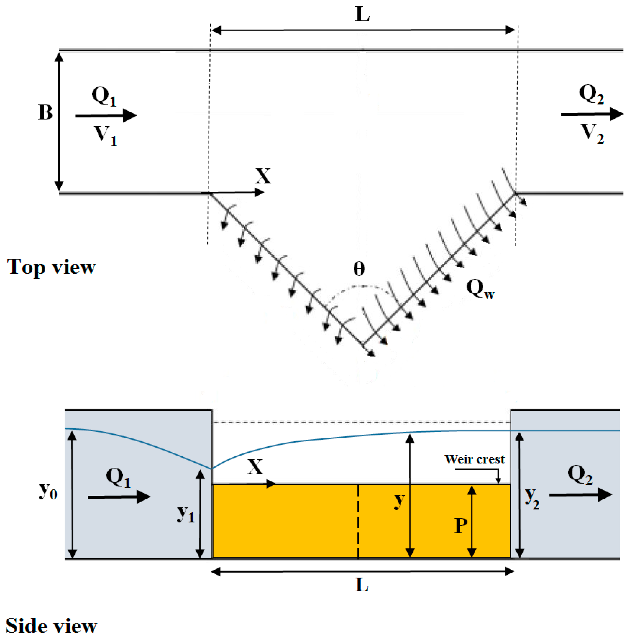
Side weirs are hydraulic structures often used for flow diversion and measurement, for irrigation and drainage purposes, and control of the floods. A side weir’s height is less than the height of the channel wall: When the water level rises, a part of the discharge overflows the weir and is diverted to another channel. One of the effective solutions to increase the efficiency of such structures is the use of a labyrinth side weir, changing the geometry of the plan and increasing the length of the weir when the crest of the side weir is not straight in a plane form. In this way, thanks to the increase in the crest length in the plan, labyrinth side weirs can overflow more discharge compared to conventional side weirs. Figure 1 shows a triangular labyrinth side weir.
According to Figure 1, y0, y, y1, and y2 are the depth of flow corresponding to Q1, the flow depth on a triangular labyrinth side weir, and the flow depth upstream and downstream of the weir (in centerline), respectively. P is the height of the side weir, B is the channel width, L is the weir opening length, and Q1 and Q2 are the flow discharge upstream and downstream of the side weir, respectively; Qw is the weir outflow discharge, V1 and V2 are the flow velocities before and after the side weir, and θ is the vertex angle of the triangular labyrinth side weir.
The hydraulic behavior of the flow in the side weir is spatially variable with discharge reduction [1]. Assuming energy conservation in the main channel, irrespective of the friction and channel slopes, the general equation of the variable spatial flow with discharge reduction can be written as follows:
where Q is discharge in the main channel, y is the depth of flow, B is the channel width, x is the distance from the beginning of the side weir, and g is the acceleration of gravity. Assuming that the specific energy across the weir is constant, the general equation of weirs can be described as
Here, dQ/dx or q is the discharge per unit length over the weir, y is the depth of flow along the channel centerline, P is the height of the weir, and CM is the discharge coefficient of the weir.
Extensive studies were carried out to obtain the relation of the discharge coefficient in a linear side weir; in most of them, the energy changes through the weir are assumed to be insignificant. Singh et al. [2] and Borghei et al. [3] performed several experiments to observe the behavior of the discharge coefficient variation over side weirs for different flow conditions, geometric characteristics, and shapes of the main channel. Coşar and Agaccioglu [4] investigated the discharge coefficient for a triangular side weir on a curved channel and highlighted that the path of maximum velocity and the secondary current created by the bend cause a much greater deviation angle toward the side weir. Other research on side weirs in a linear form include [5,6,7,8,9,10], focused on the influence of different hydraulic conditions and various geometrical parameters on flow characteristics, especially the discharge coefficient and the discharge capacity.
Non-linear side weirs, called labyrinth side weirs, with, e.g., triangular [11,12,13] or trapezoidal [14,15,16] shapes, result in a higher discharge capacity compared to a linear side weir. Aydin et al. [17] numerically analyzed the subcritical flow of trapezoidal labyrinth side weirs. The results showed that the discharge coefficient decreases as the Froude number increases, and the best side weirs had an angle of 30 degrees. Emiroglu et al. [18] examined the effects of impermeable antivortexes, installed on a trapezoidal labyrinth side weir, on the discharge coefficient and downstream scouring. The results showed that the increase in the crest length and the use of antivortex structures lead to an increase in the discharge capacity of trapezoidal labyrinth side weirs. Abdollahi et al. [19] numerically investigated flow passing over labyrinth side weirs with guiding obstacles using the OpenFOAM platform: The maximum discharge occurs when obstacles are placed downstream of the weir, perpendicular to the flow. Aydin and Ulu [20] investigated the effects of impermeable antivortexes on labyrinth side weirs: The use of an antivortex regulated the flow and increased the discharge coefficient of the side weir. Karimi et al. [21] investigated flow characteristics on asymmetric triangular side weirs and highlighted that asymmetric shapes have a higher discharge coefficient than symmetric ones.
To the best of the authors’ knowledge and according to previous studies, applying labyrinth side weirs in open channels increases the flow rate and discharge capacity of these weirs. However, it is important to consider that the flow passing through the labyrinth side weirs is associated with the vortex formation, which is more effective in labyrinth side weirs (for different Froude numbers). When this vortex formation is prevented or the risks of vortex formation are minimized, there is a greater discharge capacity. Hence, the present study aims to investigate the effect of geometric and hydraulic antivortex parameters, permeable and impermeable, on discharge capacity considering six different shapes and weir heights using the CFD technique. The paper is organized as follows: First, an overview of the work and research done on hydraulic flow through side weirs and on the use of labyrinth side weirs as a means to increase efficiency is presented; second, the hydraulic and geometric characteristics of the models studied and the numerical setup of the simulations carried out are described. Afterwards, the numerical model is validated with experimental results, and the hydraulic performance of the antivortex inside a triangular labyrinth side weir is analyzed. The article ends with a conclusion and a discussion on the numerical results obtained.
2. Materials and Methods
2.1. Input Parameters for Numerical Models
The calibration data provided by Kabiri Samani et al. [12] allow for a comparison of the numerical model and laboratory test results in this study. In Table 1, the geometric characteristics of the tested triangular labyrinth side weir are presented. The laboratory model used is a horizontal rectangular channel with a length, width, and height of 6.5, 0.4, and 0.5 m, respectively. The triangular labyrinth side weir is modeled as a single cycle, with weir angles of 75 degrees and a ratio of L/B = 1.31 (L: The weir opening length; B: Channel width). Although the length of the experimental flume was 6.5 m, the present numerical study reduces it to 5 m to improve computational performance and reduce the number of overall cells.
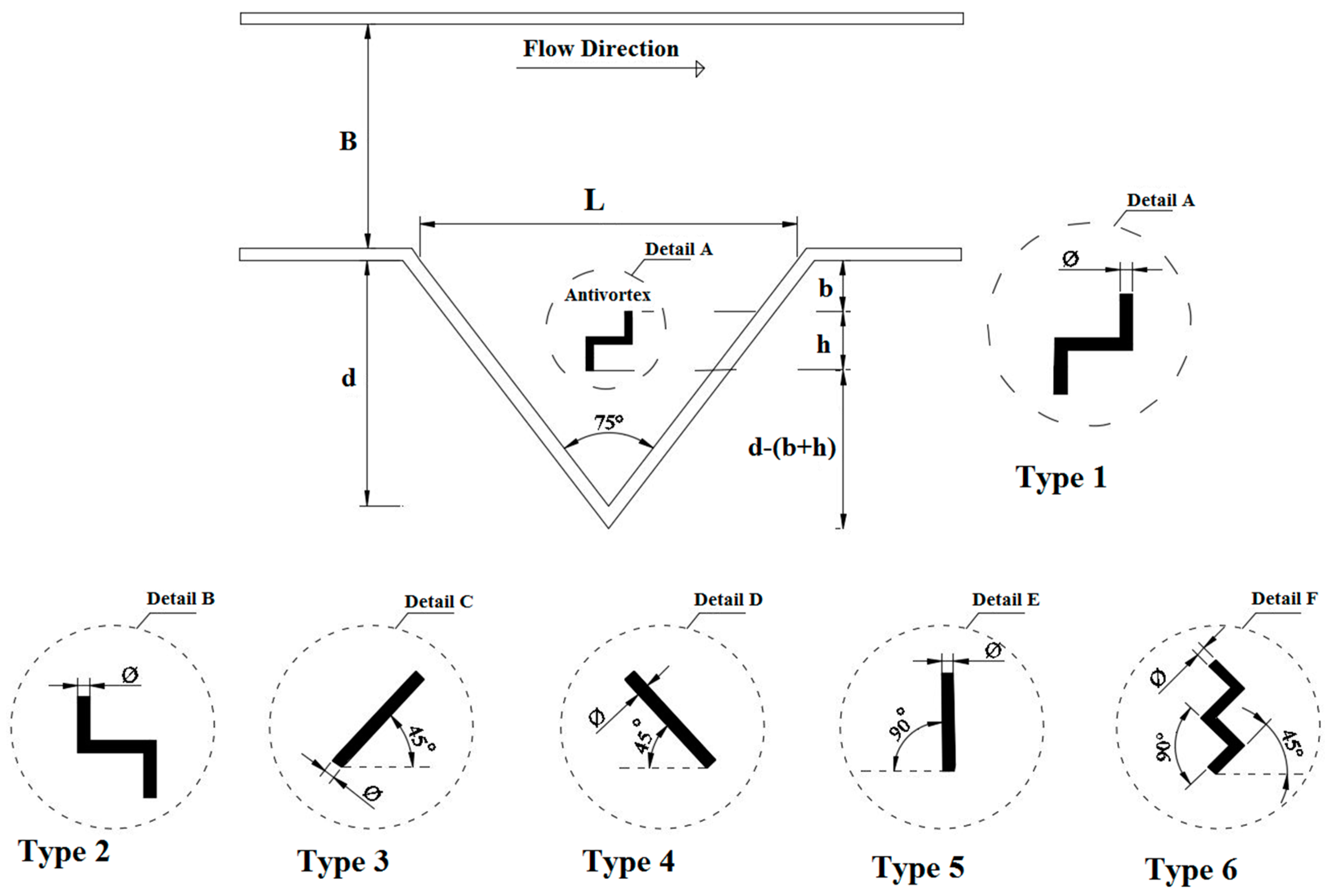
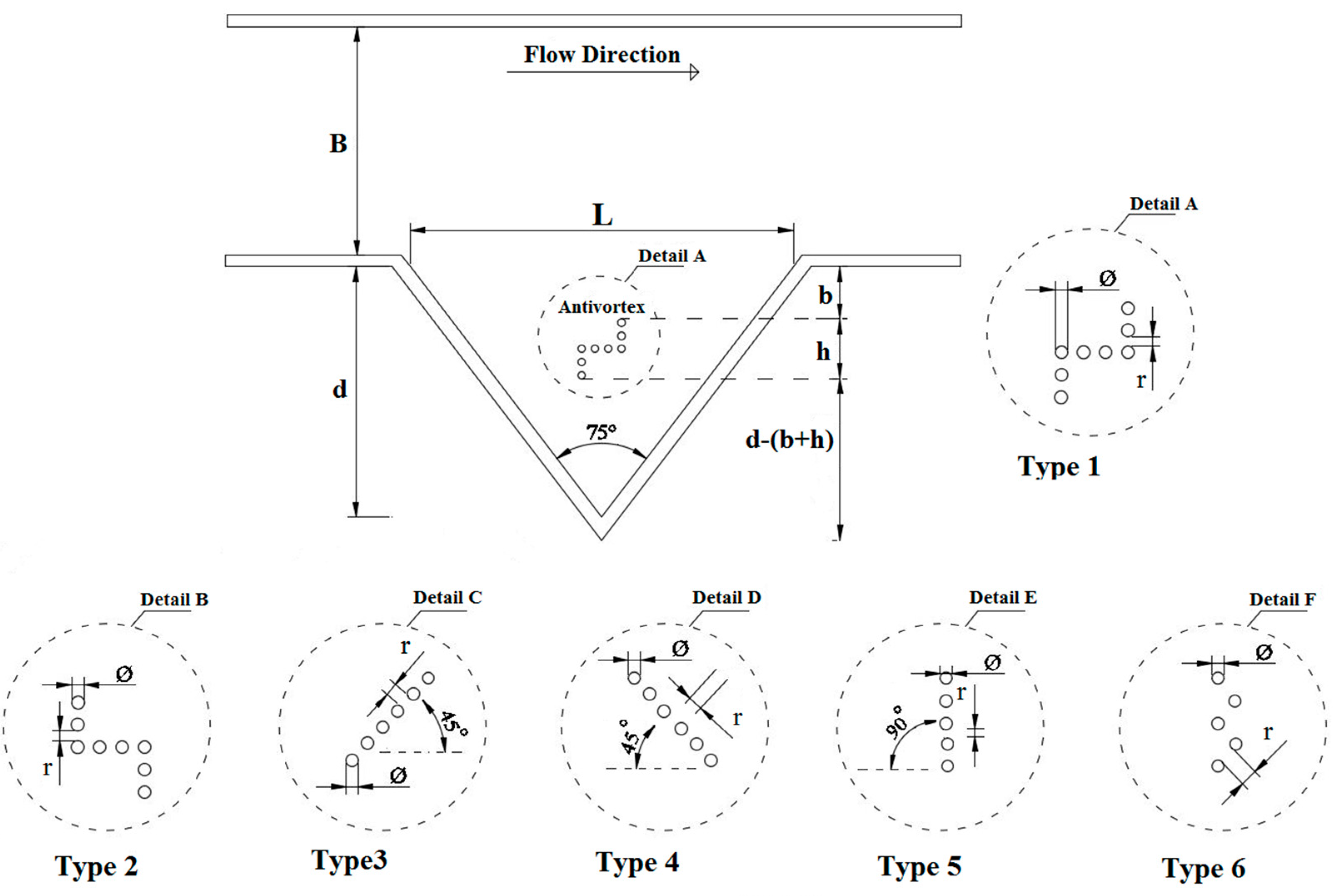
As a first step, the simulation results, such as discharge coefficient and the water surface profile in the absence of antivortexes, were validated with the laboratory results from Esmaili [22] and Kabiri Samani et al. [12]; then, by placing the antivortexes inside the triangular labyrinth side weir, in permeable and impermeable modes, with three different heights of 0.078, 0.117, and 0.156 m, their performances were evaluated in terms of discharge coefficient. A total of 185 simulations was analyzed. The hydraulic conditions of the flow and the geometric characteristics of all the simulated models are presented in Table 2 and Figure 2.
2.2. Computational Fluid Dynamics (CFD)
FLOW-3D® is a CFD program for modeling multi-physics flow problems and simulates flow, turbulence, bed load, and suspended load under different boundary conditions [23]. FLOW-3D® bases its strategy to model and track the free surface on the volume of fluid (VOF) method [24]. This software uses the finite volume method to solve the RANS equations (Reynolds Average Navier-Stokes) in a Cartesian, staggered grid. As follows, model governing equations are briefly described in the form of tensor notations. The conservation of mass (continuity equation, assuming incompressibility of the flow) is written as
The conservation of momentum (Navier–Stokes equations, assuming constant fluid properties and incompressible Newtonian fluid) is expressed as
where ui and xi are velocity and position vectors, t denotes the time, p is pressure, ρ is density, g is gravitational acceleration, and tij refers to the viscous stress tensor, and can be expressed by
in which μ is molecular viscosity, and sij is the strain-rate tensor, which can be defined as follows:
Note that sij = sji, so that tji = tij for simple viscous fluids [25]. The VOF transport equation is expressed by the following:
Here F is the fraction function. In particular, F = 0 when a cell is empty, and F = 1 when a cell is full [23]. The free surface is located at a position pertaining to intermediate values of F (usually F = 0.5, but another intermediate value may be defined by the user).
2.3. Turbulence Model
Using Reynolds decomposition, we can apply into the Navier-Stokes equations and obtain averaging Navier-Stokes equations. The Boussinesq hypothesis is used to relate the Reynolds stresses tensor () to the mean velocity gradients using an eddy viscosity by the following equation:
where Ui is the mean velocity component in a Cartesian coordinate system, xi is the Cartesian space (i, j, k), εij is the eddy viscosity tensor, δij is the Kronecker delta, and k is the turbulent kinetic energy [26]. In this study, the chosen turbulence model was RNG k-ε, since, in Flow Science, Inc. [23] and Chero et al. [27], it is mentioned that the RNG k-ε model has wider applicability than the standard k-ε and is usually the best choice. The RNG k-ε turbulence model has an additional term in its equation that improves the accuracy of rapidly strained and swirling flows; the results of numerical studies on simulating flow on side weir and hydraulic structures [28,29,30,31,32,33,34] also show its accuracy. This model represents a modified version of the k-ε standard model [35].
The adopted scheme is a two-equation model. In particular, the first equation (Equation (9)) is called turbulent kinetic energy (k). The second equation (Equation (10)) is the turbulent dissipation rate (ε), which determines the rate of kinetic energy dissipation.
Here, Gk is the generation of turbulent kinetic energy caused by the average velocity gradient, Gb is the generation of turbulent kinetic energy caused by buoyancy, and Sk and Sε are source terms. αk and αε are inverse effective Prandtl numbers for k and ε, respectively. μeff is the effective viscosity. μeff = μ + μt, μt being the eddy viscosity.
For the above equation,
The constant values for this model are [35] Cµ = 0.0845, C1ε = 1.42, C2ε = 1.68, C3ε =1.0, σk = 0.7194, σε = 0.7194, η0 = 4.38, and β = 0.012.
2.4. Computational Mesh and Boundary Conditions
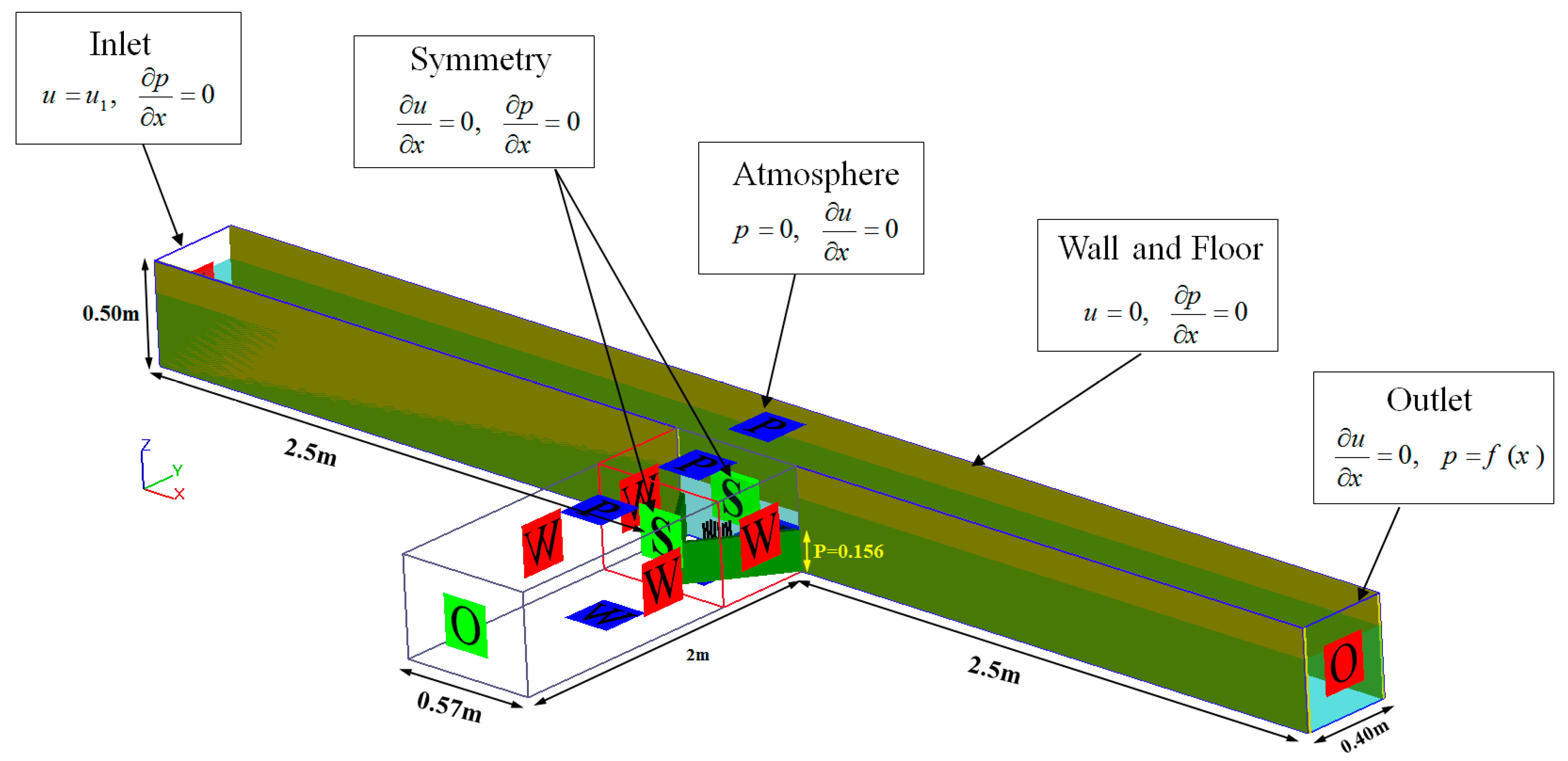
The side weir setup was performed by inserting a sterolithography (STL) file. The determination of the representative boundary conditions is important for numerical simulation and hydraulic analysis. According to the experimental conditions in Kabiri Samani et al. [12], the following boundary conditions were employed (Figure 3):
- Specified pressure (P) was used for the input flow corresponding to the inlet water depth and outlet (O) conditions for flow for the downstream boundary.
- The lower Z (Zmin) and both of the side boundaries were treated as a rigid wall (W). No-slip conditions were applied at the wall boundaries. No-slip is defined as zero tangential and normal velocities (u = v = w = 0). With a no-slip boundary, it is assumed that a law-of-the-wall type profile (the average velocity of a turbulent flow at a certain point is proportional to the logarithm of the distance from that point to the boundary of the fluid region) exists in the boundary region [23,36]. The no-slip boundary condition was imposed on the wall, and friction was neglected. Thus, no roughness is imposed at the wall boundary [23].
- An atmospheric boundary condition was set to the upper boundary of the channel. This allows the flow to enter and leave the domain, as null von Neumann conditions were imposed to all variables except for pressure, which was set to zero (i.e., atmospheric pressure).
- A symmetry boundary condition (S) is imposed at the inner boundaries as well, which allowed for flow-through. In a symmetry boundary condition, no shear stresses are calculated across the boundary [23].
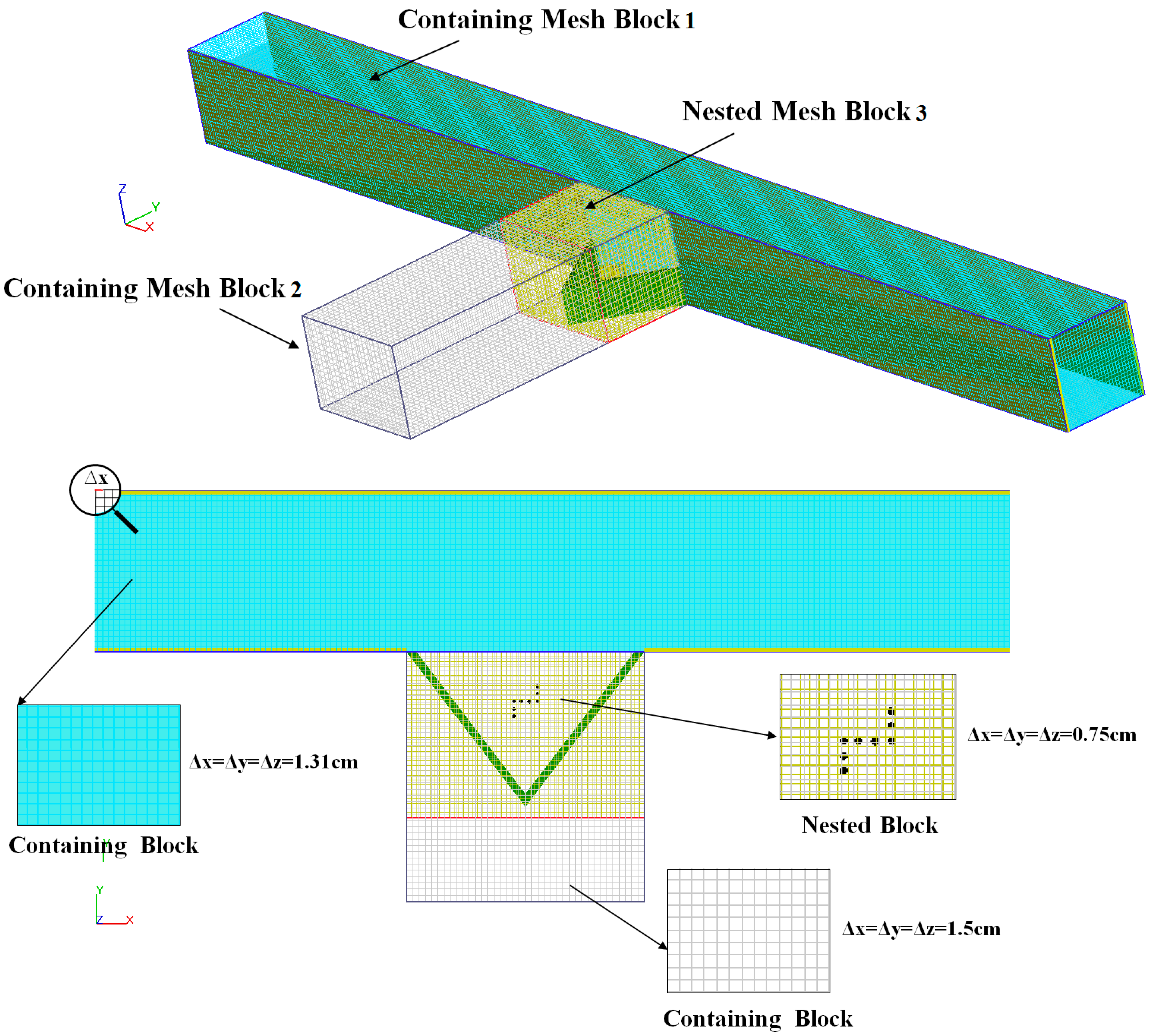
FLOW-3D® implements “free gridding” using the Fractional Area Volume Obstacle Representation (FAVOR) [23,30], the mesh being essential for an accurate solution. In this case, a containing mesh block was created for the entire spatial domain, and a nested mesh block was then built, with refined cells for the area of interest, where an antivortex was located inside the triangular labyrinth side.
Several computational meshes and the grid convergence index (GCI) were utilized to select the appropriate mesh, which is a widely accepted and recommended method for estimating discretization error that has been applied to several CFD cases [37,38,39,40]. The methodology is described in Roache [41] and was developed following the Richardson extrapolation method of Celik et al. [42]. Three different meshes with fine, medium, and coarse cells, consisting of 2,798,910, 1,975,870, and 875,632 cells in total, respectively, were used to examine the effect of the grid size on the accuracy of the numerical results. Table 3 summarizes some details of the three computational grids. Cell size was considered the minimum refinement ratio, (r = Gcoarse/Gfine), which was 1.3, as recommended by Celik et al. [42].
A grid convergence index (GCI), the most common and reliable technique for quantification of discretization uncertainty in numerical results, was determined for the computed free surface profiles on the three grids [41]. Using the Richardson error estimator to compare the three grids, the fine-grid convergence index is defined as
where E32 = (us2 − us3)/us2 is the approximate relative error between the medium and fine grids; us2 and us2 are the medium and fine grid solutions for the free surface profiles, respectively; p is the local order of accuracy. For the three-grid solutions, p is obtained by solving
where e21 = us2 − us1, e32 = us3 − us2, r21 = G2/G1 and is the grid refinement factor between a coarse and medium grid, and r32 = G3/G2 and is the grid refinement factor between a medium and fine grid (for the present three-grid comparisons, G1 < G2 < G3). Table 4 shows a summary of the GCI calculations. The obtained results indicate the mesh convergence with the GCI equal to 3.87%.
Once the mesh convergence analysis was performed, the mesh consisting of a containing block with a cell size of 1.31 m and a nested block of 0.75 m was chosen (refer to Figure 4 for modeling details).
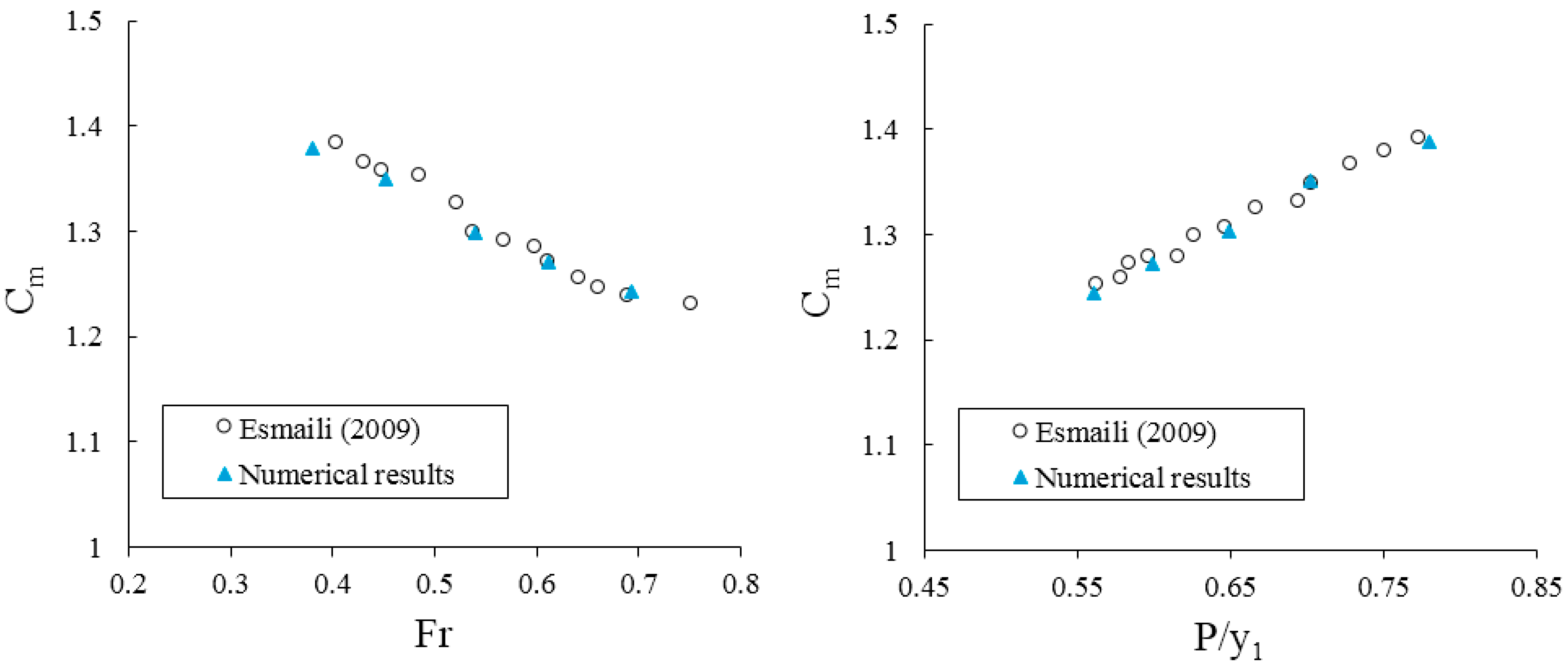
For verifying the obtained results from the numerical modeling, the discharge coefficients obtained from the numerical simulations are compared with the experimental data by Esmaili [22]. According to Figure 5, the results show that the trend and the discharge value obtained from numerical modeling well agree with the experimental data. The average error of numerical modeling is 2.8%.
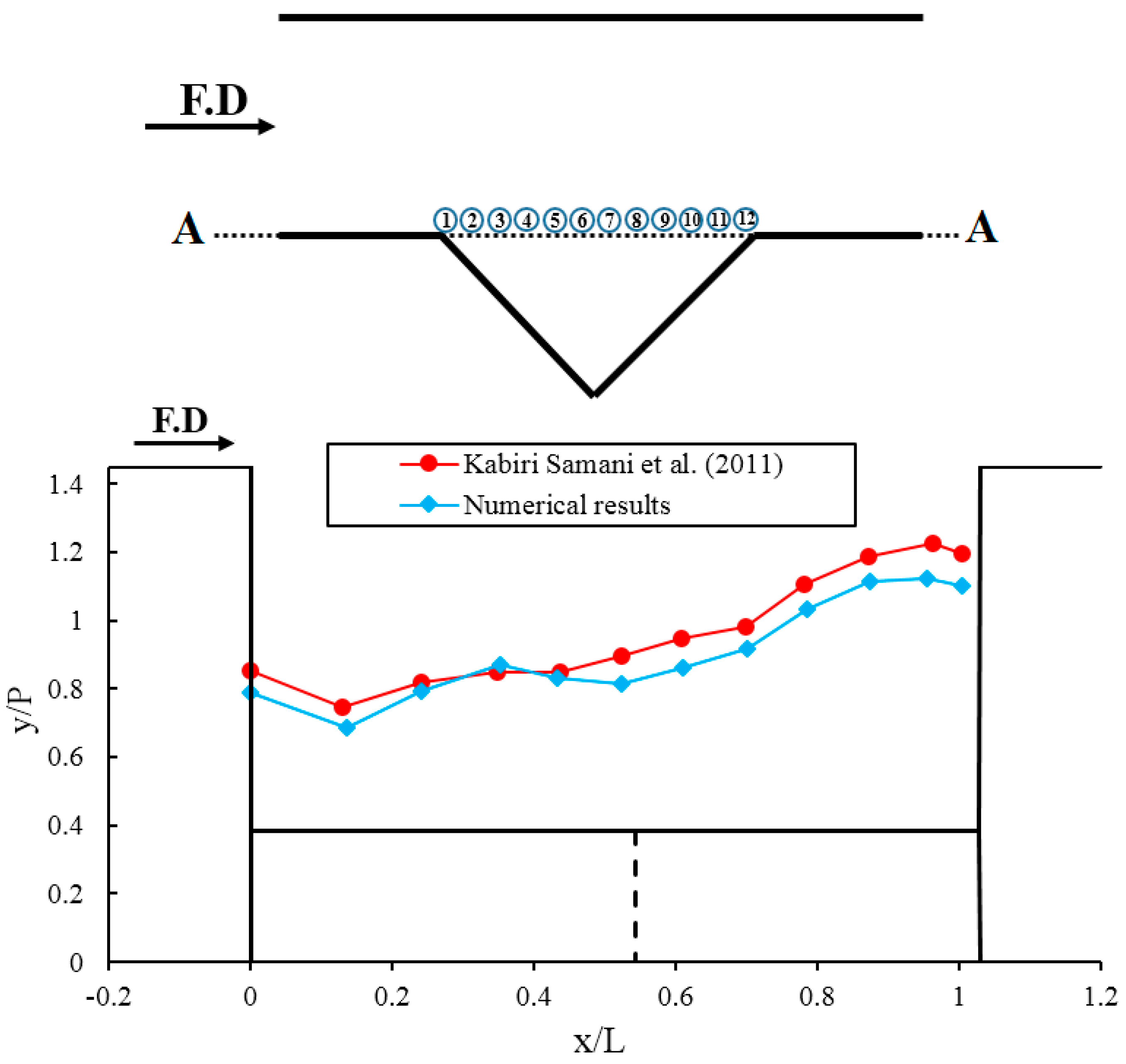
The free surface profiles over the triangular labyrinth side weir from numerical and experimental model by Kabiri Samani et al. [12] for the inlet Fr = 0.38 are shown in Figure 6. Comparisons of the experimental and numerical results in accordance with the water free surface profiles on the axis A-A are illustrated in Figure 6.
In this figure, the vertical axis is the ratio of the water depth to the height of the side weir (y/P), and the horizontal axis is the dimensional ratio of the location in the direction of the channel length over the weir opening length (x/L). A good agreement can be observed in the trend between the results of the experimental and numerical models, and the maximum discrepancies of the water free surface profiles is 3.1%, which confirms the ability of the numerical model to predict specifications of flow over the triangular labyrinth side weir. As is shown in Figure 6, the water surface level decreases at the beginning of the triangular labyrinth side weir, and this level rises rapidly to the end of the side weir. According to the studies of El-Khashab and Smith [43], and Emiroglu and Kaya [14], the cause of this phenomenon is the effect of the current deviated from the main channel and the entrance to the side weir.
2.5. Near Wall Treatment
Usually, turbulence models are accurate and valid only for fully turbulent flows. However, near the wall, the flow is almost laminar, and the turbulent stress hardly works, especially for the viscous sublayer region [44]. As a result, the traditional turbulence models do not work well here. Currently, there are two different methods (the near wall modeling method and the wall function method) to solve the problem. Both methods involve a dimensionless distance y+ and the distance of the first grid point from the wall (yp) as a function of shear velocity () and the kinematic viscosity of the fluid (υ):
The near wall modeling method directly utilizes the low Reynolds number turbulence model with much finer grids near the wall to deduce parameters in the viscous sublayer. It requires that the grid point of the first layer should be arranged within the viscous layer (y+ < 1). The wall function method does not directly deduce the viscous sublayer, but arranges the grid point of the first layer within the log law region (30 < y+ < 200∼400) and then relates the viscous layer to the log law region with empirical formulas [45]. Compared with the near wall modeling method, the wall function method does not need to specifically compact the grid near the wall, but saves much more computation time with higher efficiency. In view of the unique grid generation technology in the FLOW-3D software, as shown in Figure 4, the grid can be flexibly adjusted to embed into the walls of the numerical model. In addition, as shown in Table 5, two different grid systems are arranged to fill the blocks to evaluate the effect of the grid size upon the numerical results. It can be noticed that the dimensionless y+ in all grid systems ranges from 54 to 79 and confirms the requirement of the wall function method. The upstream Reynolds number varies between 11,353 and 35,471.
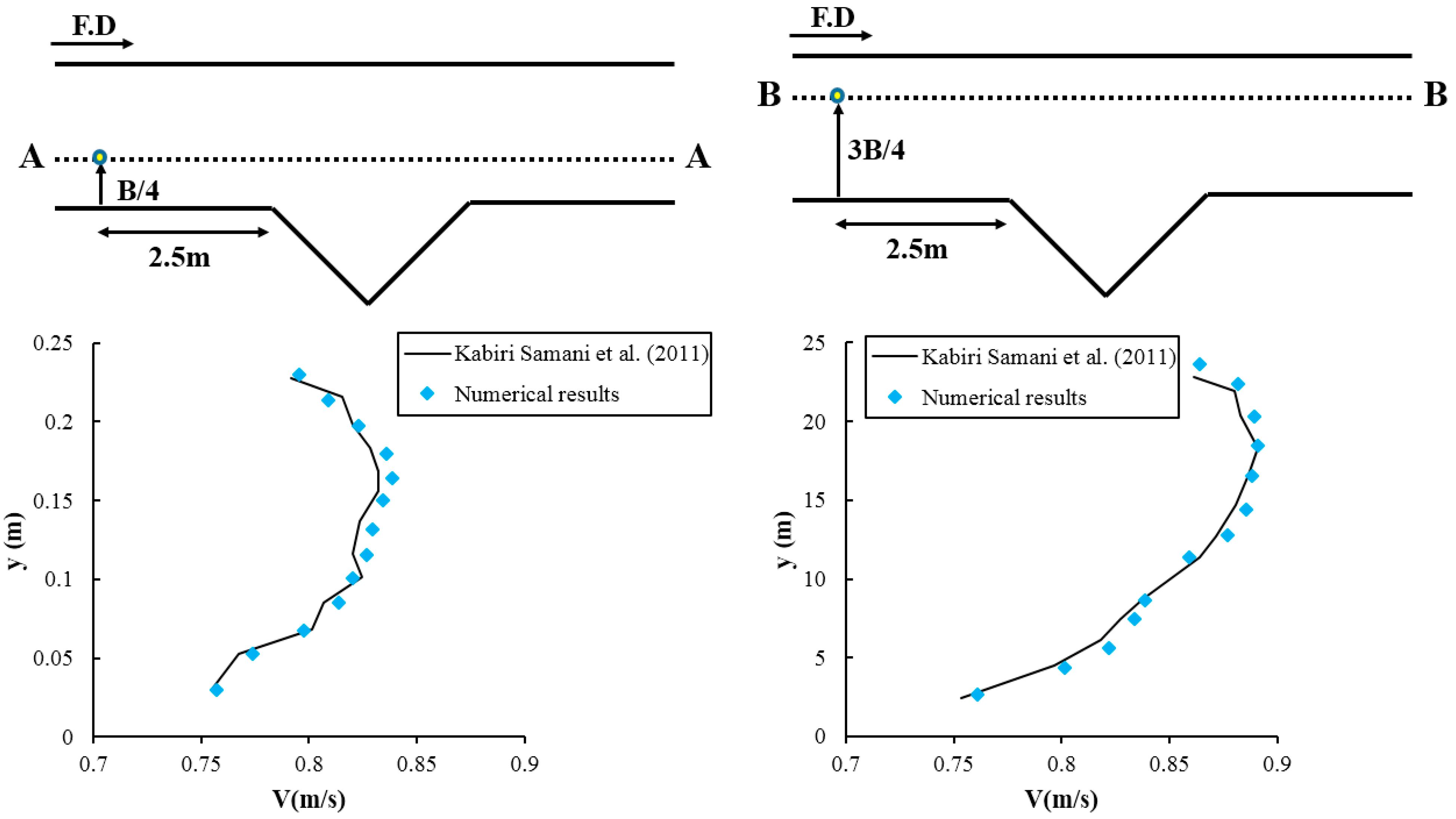
Regarding time discretization, the time-step size was automatically adjusted by the code, using a Courant-type stability criterion to improve model efficiency with a reduction in computational time and to minimize numerical divergence risk (time steps between 0.0011 s and 0.0014 s). The turbulence length scale (LT) is a quantitative physical parameter that relates to the size of large eddies that contain the turbulent energy of the stream [44]. In the FLOW-3D model, the maximum turbulent length scale is a user-defined parameter that represents an estimate to the actual length scale for flow turbulence. Furthermore, this parameter could be estimated at 0.07 times of B for fully developed flows, where B is the flume/channel width [46]. The velocity of flow in the main channel is controlled during the solution to ensure the solution’s convergence and fully establishes the conditions imposed on the model (see Figure 7). The steady-state condition is achieved for all of the inlet Fr values with a simulation time of 25 s. The steady state message was obtained from the solver. The computational time for the simulations was between 9 and 11 h using a personal computer with an eight-core CPU (Intel Core i7-7700K @ 4.20GHz and 16 GB RAM).
3. Results and Discussion
3.1. Hydraulic of Flow Passing over the Triangular Labyrinth Side Weir with an Antivortex
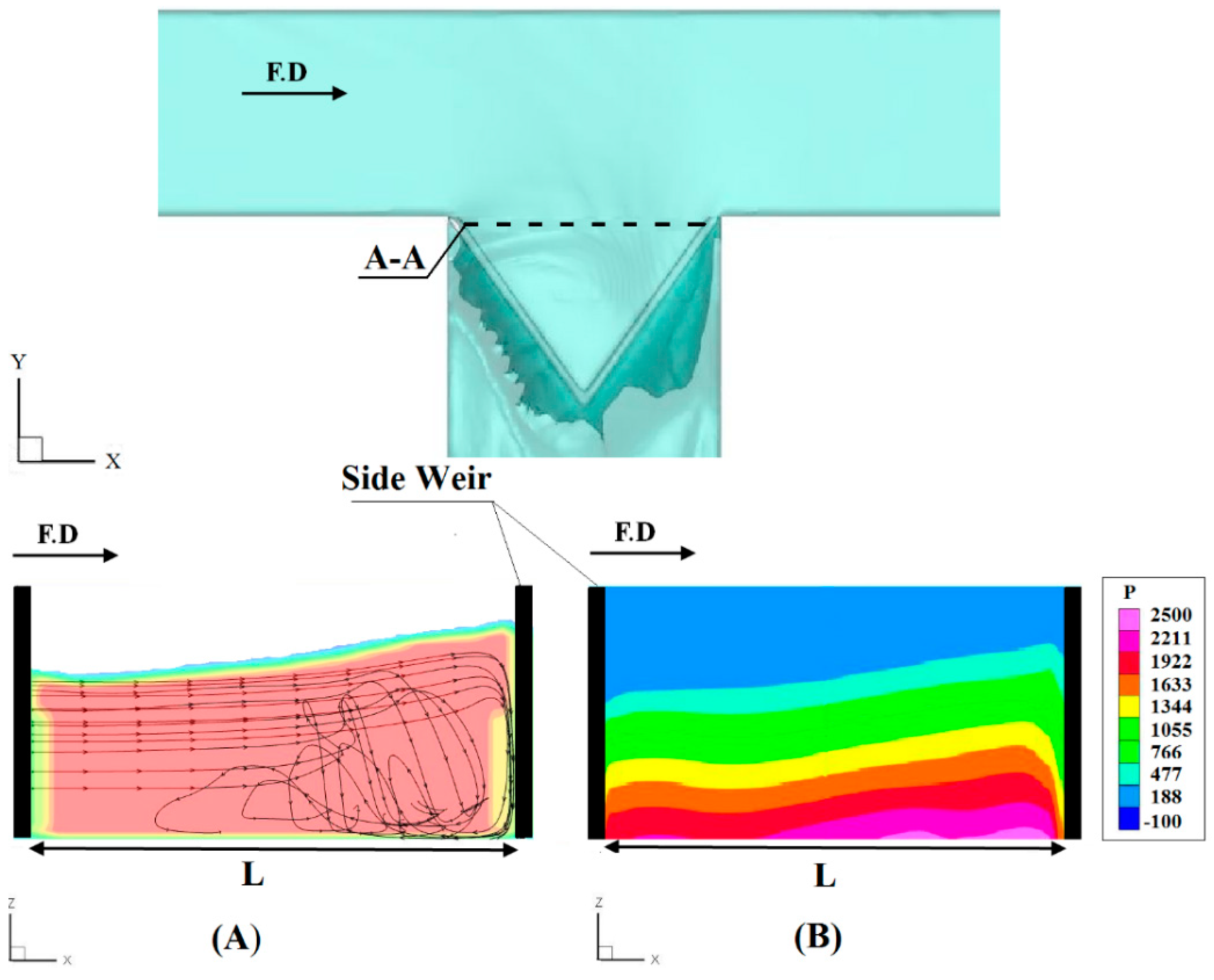
According to Figure 8, by changing the flow path from the main channel to the side weir, the current entering the side weir causes larger vortexes. The water surface level changes along the opening length of the triangular labyrinth side weir are due to the effect of the secondary flow created by the lateral flow that leads to the formation of a separation zone and reverse flow area at the end of the side weir.
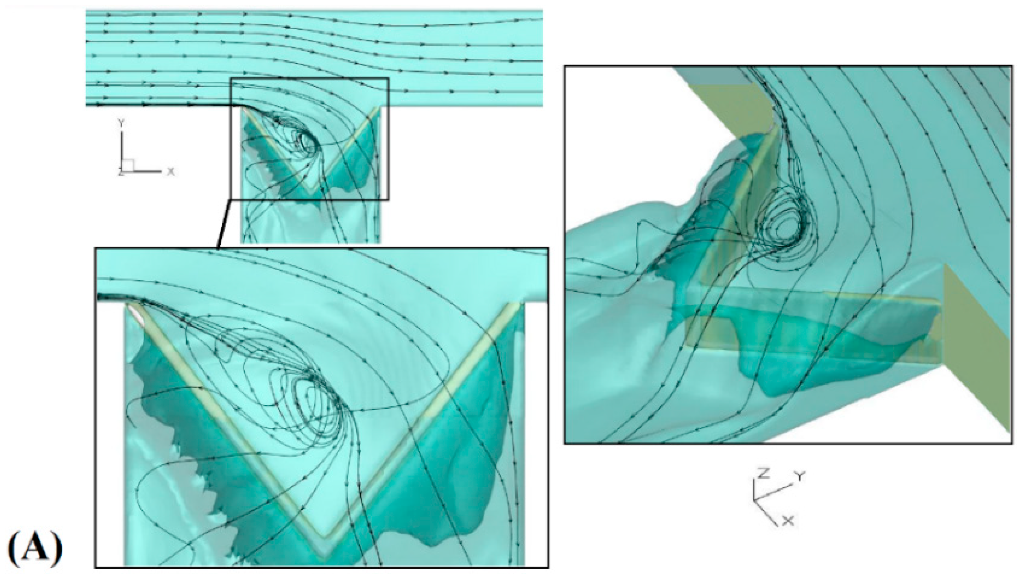
Figure 9 shows the lateral flow over the triangular labyrinth side weir without and with an antivortex. It can be seen that, inside the triangular labyrinth side weir, vortexes are mainly due to the change in flow direction and to the collision with the triangular wall. These vortexes disrupt the flow direction on the side weir and reduce the discharge capacity.
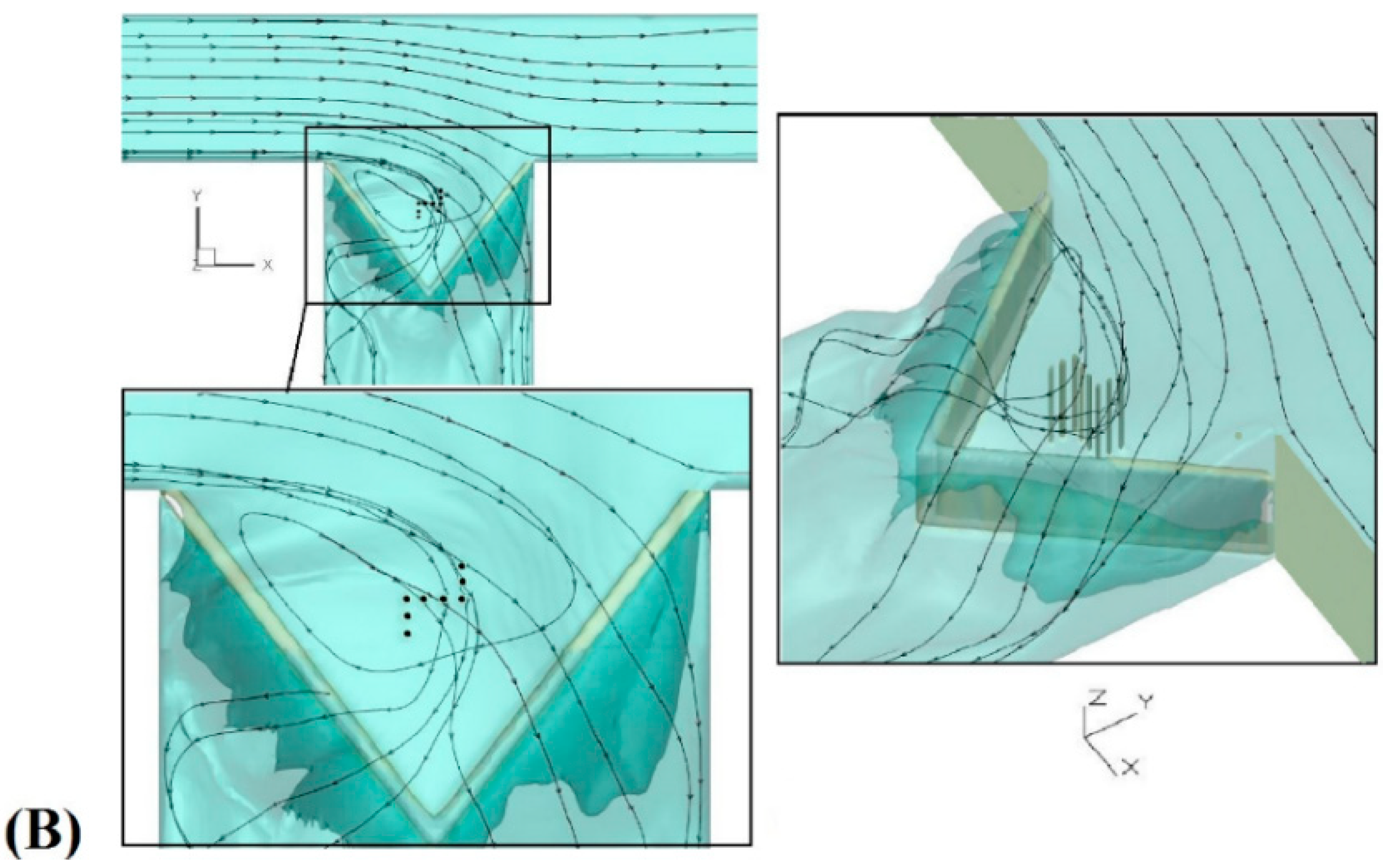
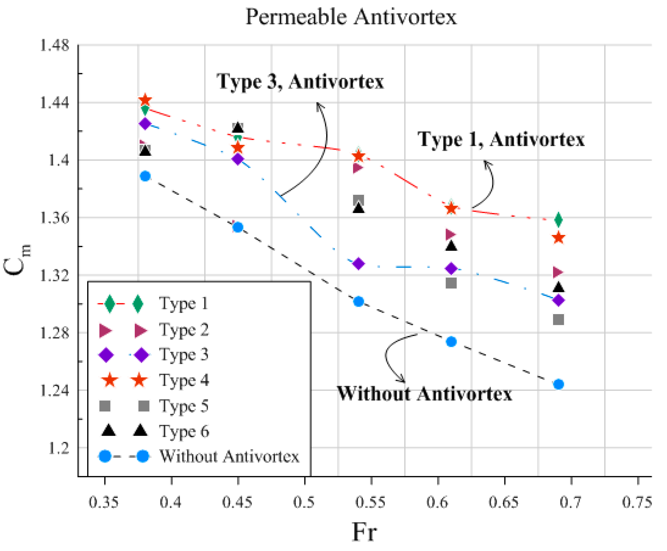
The use of antivortexes inside the triangular labyrinth side weir, despite creating an obstacle in the flow, reduces the vortexes and flow velocity inside and near the apex of the side weir, leading to a more uniform lateral flow. Figure 10 shows a comparison of the discharge coefficient of the lateral flow passing over the triangular labyrinth side weir using different types of antivortexes.
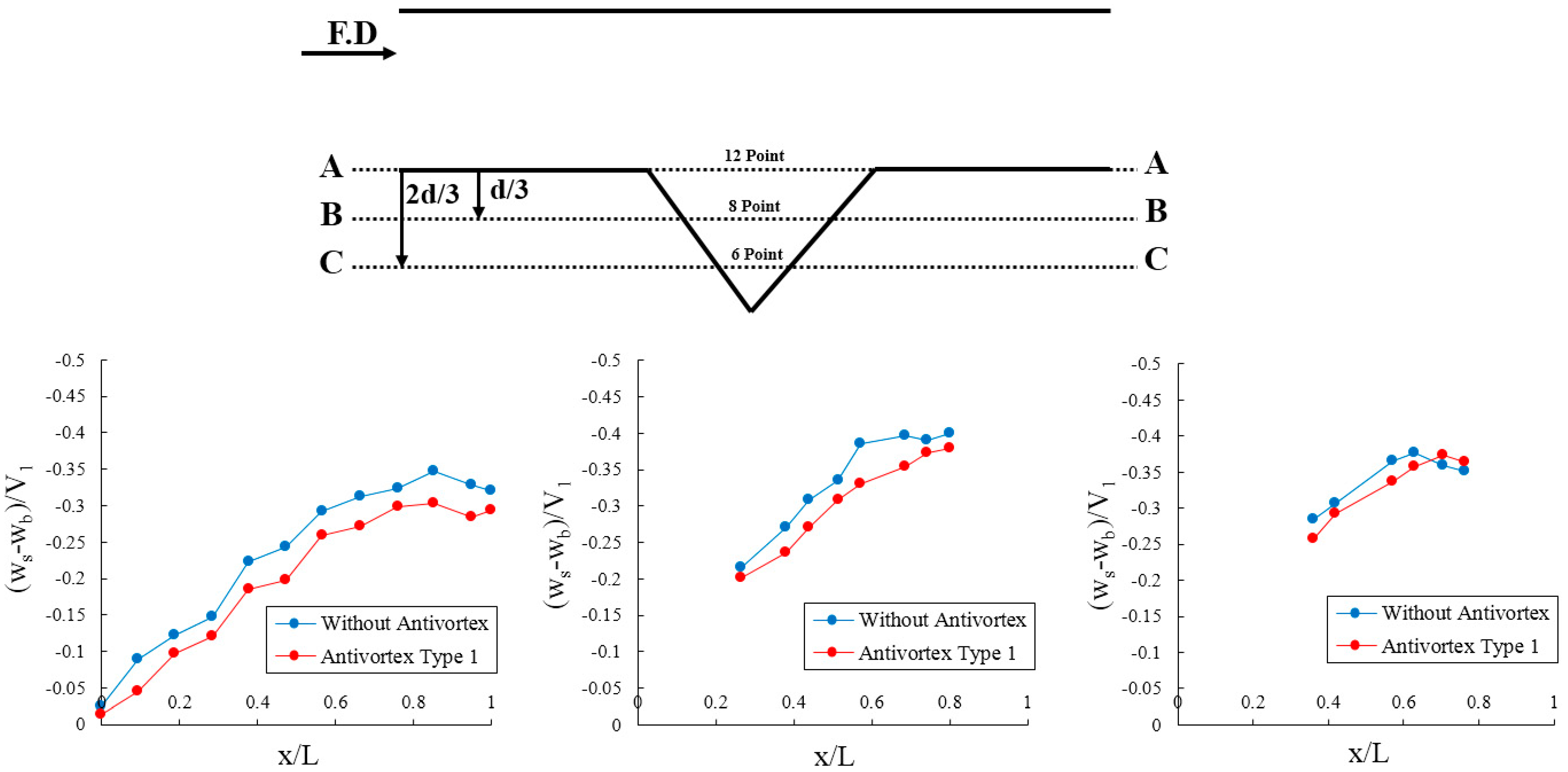
The antivortexes increased the discharge coefficient of the lateral flow passing over the triangular labyrinth side weir. The amount of increase depends on the geometric shape of the antivortex structure, with an average value of 7%. Among the antivortexes used in this study, Type 1 had the best performance, increasing the discharge coefficient by up to about 11%, while Type 3 increased it by 3% and had the smallest effect among all other types (Figure 10). By increasing the Froude number, the performance of the antivortexes improves: The performance of the side weir reduces due to local submergence, while the intensity of the secondary motion created by lateral flow increases. Thus, the antivortexes were able to increase the discharge coefficient in the side weir by reducing the vortexes. For example, when Fr = 0.38, the antivortexes increased the discharge coefficient of the triangular labyrinth side weir on average by 4.3%; when Fr = 0.69, this increase was about 10.4%. The secondary flow intensity is a function of (ws − wb)/V1, where ws and wb are the transverse velocities near the surface and near the bed, and V1 is the velocity at the upstream of the side weir. In Figure 11, the intensity of the secondary motion is shown at the side weir with three sections of the A-A, B-B, and C-C axes. With regard to this figure, the secondary flow intensity is increased along the triangular labyrinth side weir at all sections, and maximum intensity occurred at the downstream end of the side weir. The secondary flow intensity near the apex of the side weir is greater than at the beginning of the side weir. The antivortexes thus reduce the intensity of secondary flow in all cases.
3.2. The effect of Antivortex Permeability and Impermeability
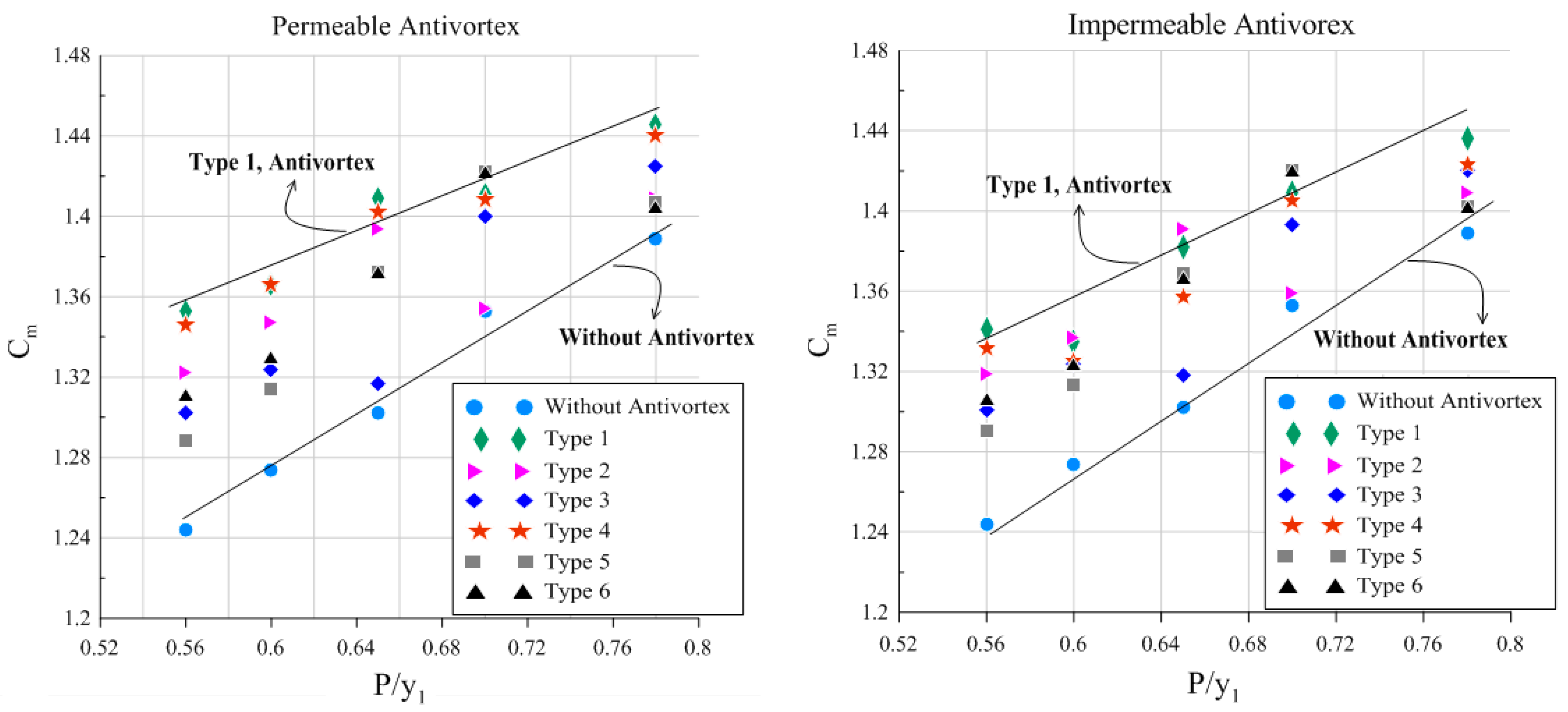
Permeable antivortexes outperformed the impermeable type: The average increase in the discharge coefficient is 3%. This is due to the vortex reduction and flow path obstruction effect of the antivortex inside the triangular labyrinth side weir. The best performance, in terms of increasing the discharge coefficient, are attributed to Type 1 followed by Type 4: Permeable Antivortex Type 1 increased the discharge coefficient by about 11% compared to the case without an antivortex.
Figure 12 shows the variation in discharge coefficient (Cm) with P/y1 (P: Side weir height; y1: The depth of flow upstream of the triangular labyrinth side weir) for the triangular labyrinth side weir with permeable and impermeable antivortexes.
3.3. Flow Velocity and Pressure over the Triangular Labyrinth Side Weir with an Antivortex
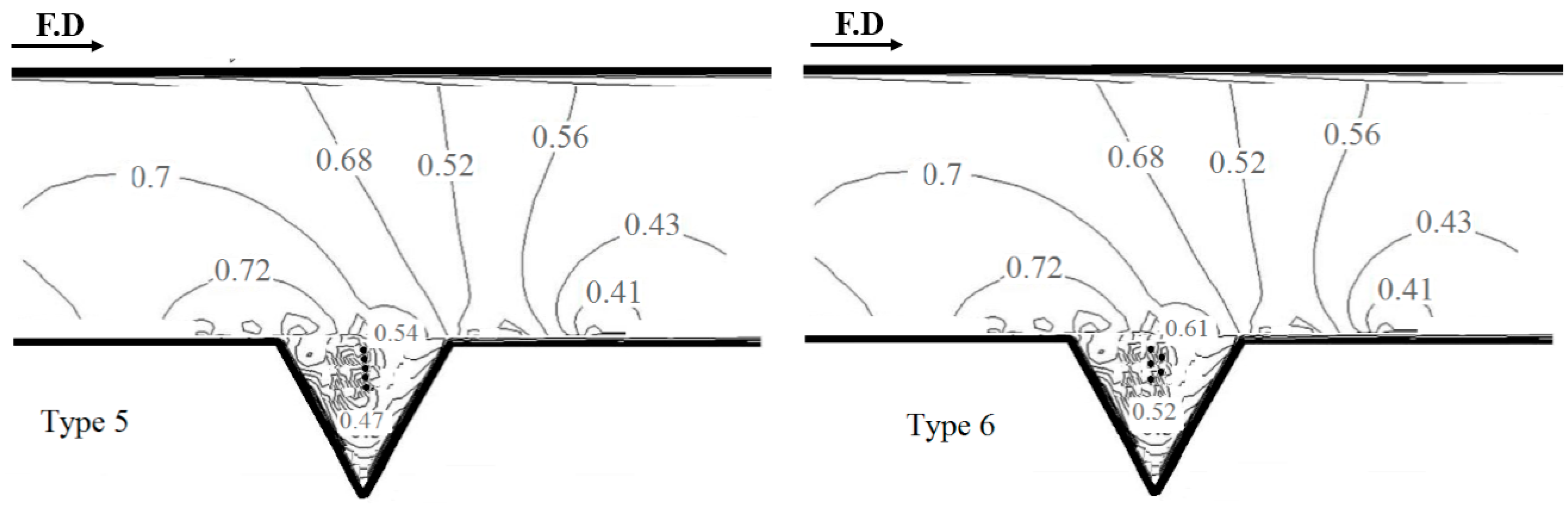
The intensity of secondary flow created by the lateral flow is defined as the ratio of the mean kinetic energy of the lateral motion to the total kinetic energy of the main flow at a given cross section. The velocity of the main flow as well as the lateral flow is shown in Figure 13. The antivortex reduces the flow velocity inside the side weir. When the flow velocity reduces, the intensity of the secondary flow occurring inside the side weir decreases, and a significant effect on the discharge performance is observed.
Figure 13 shows that Permeable Antivortex Type 1 performs better than the impermeable antivortexes by further reducing the flow velocity and making the flow more uniform. Comparing the antivortex shapes indicates that Type 1 outperforms the other antivortexes by increasing the discharge coefficient of the triangular labyrinth side weirs (see Figure 14).
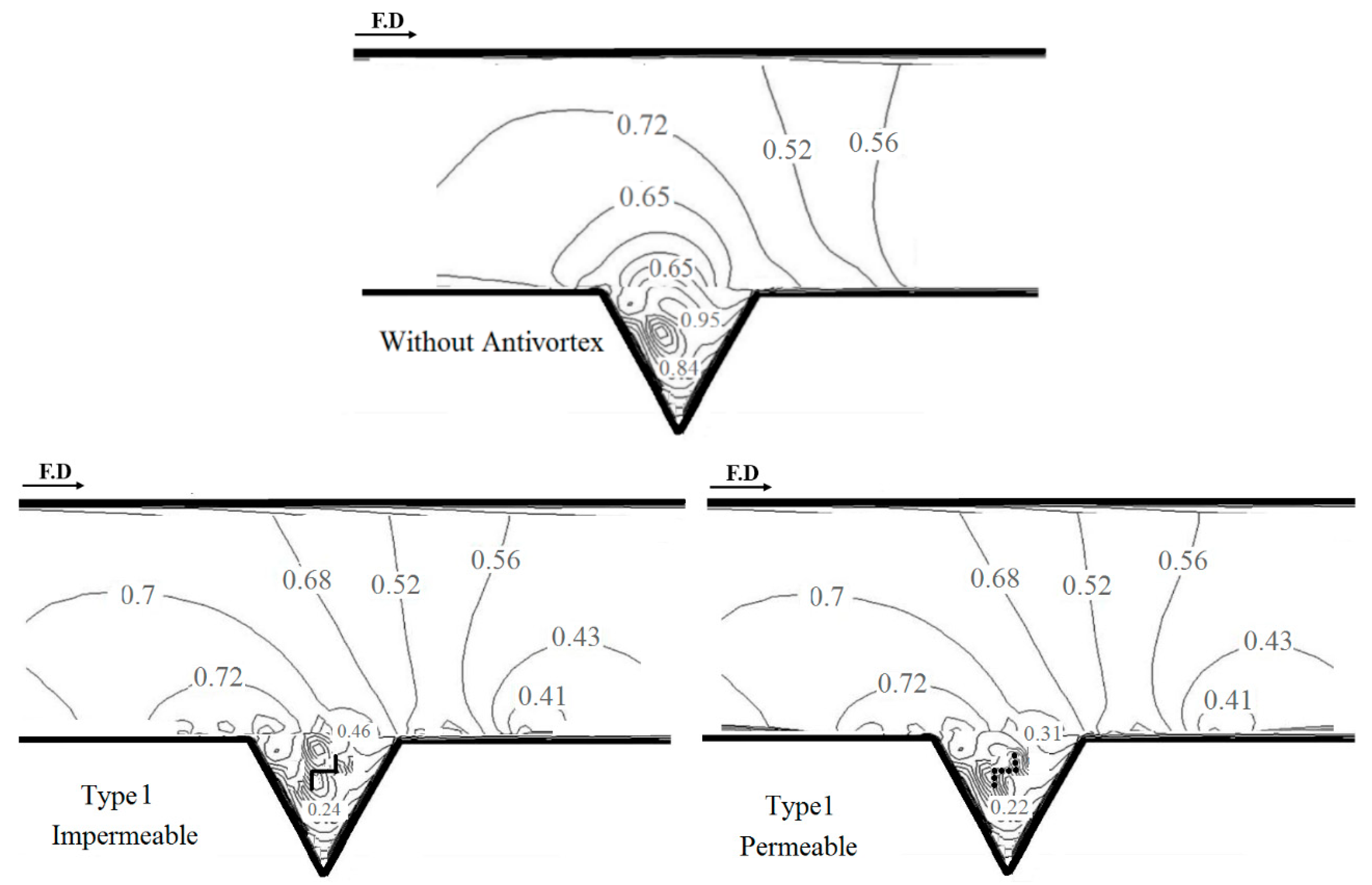
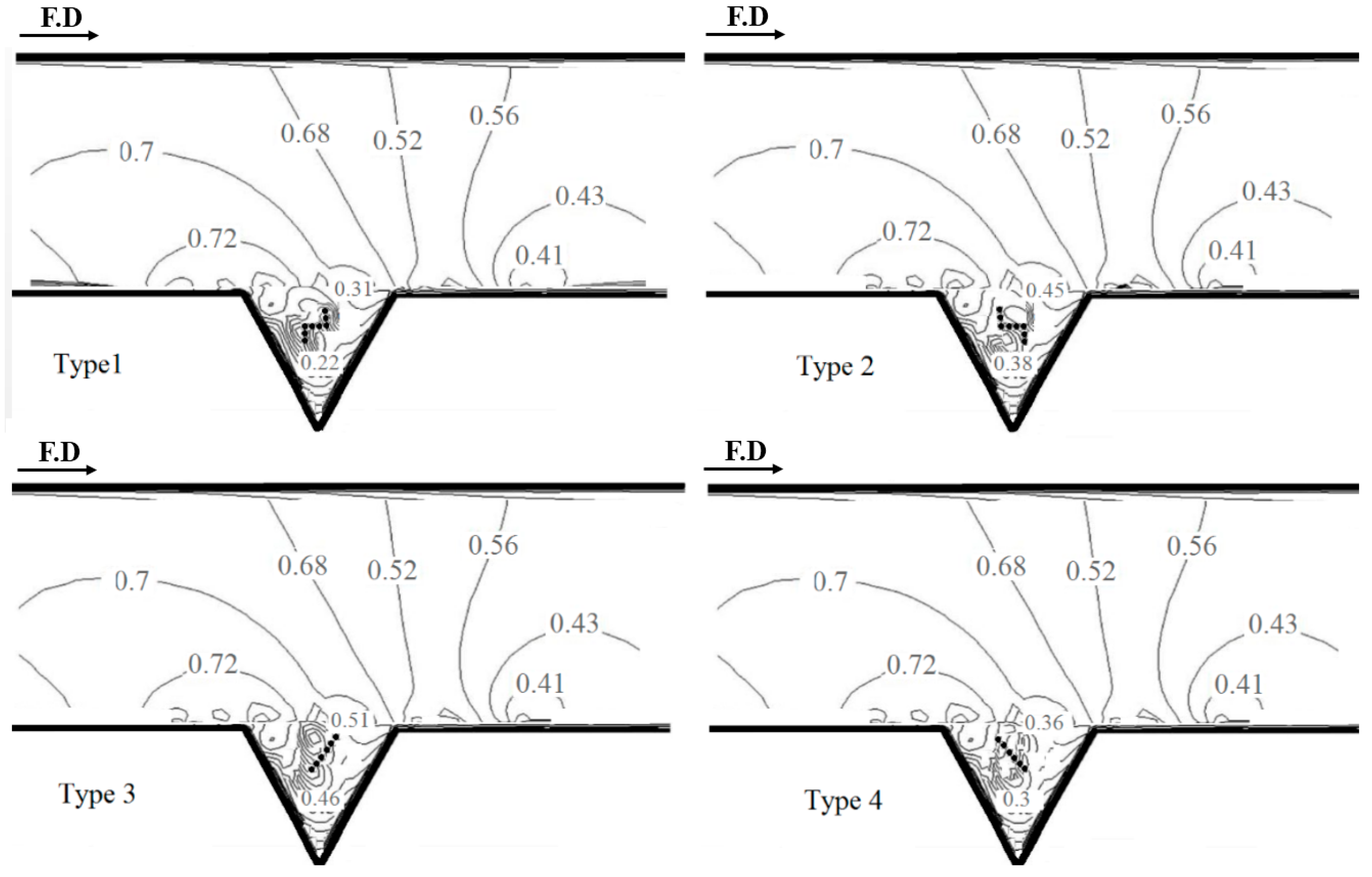
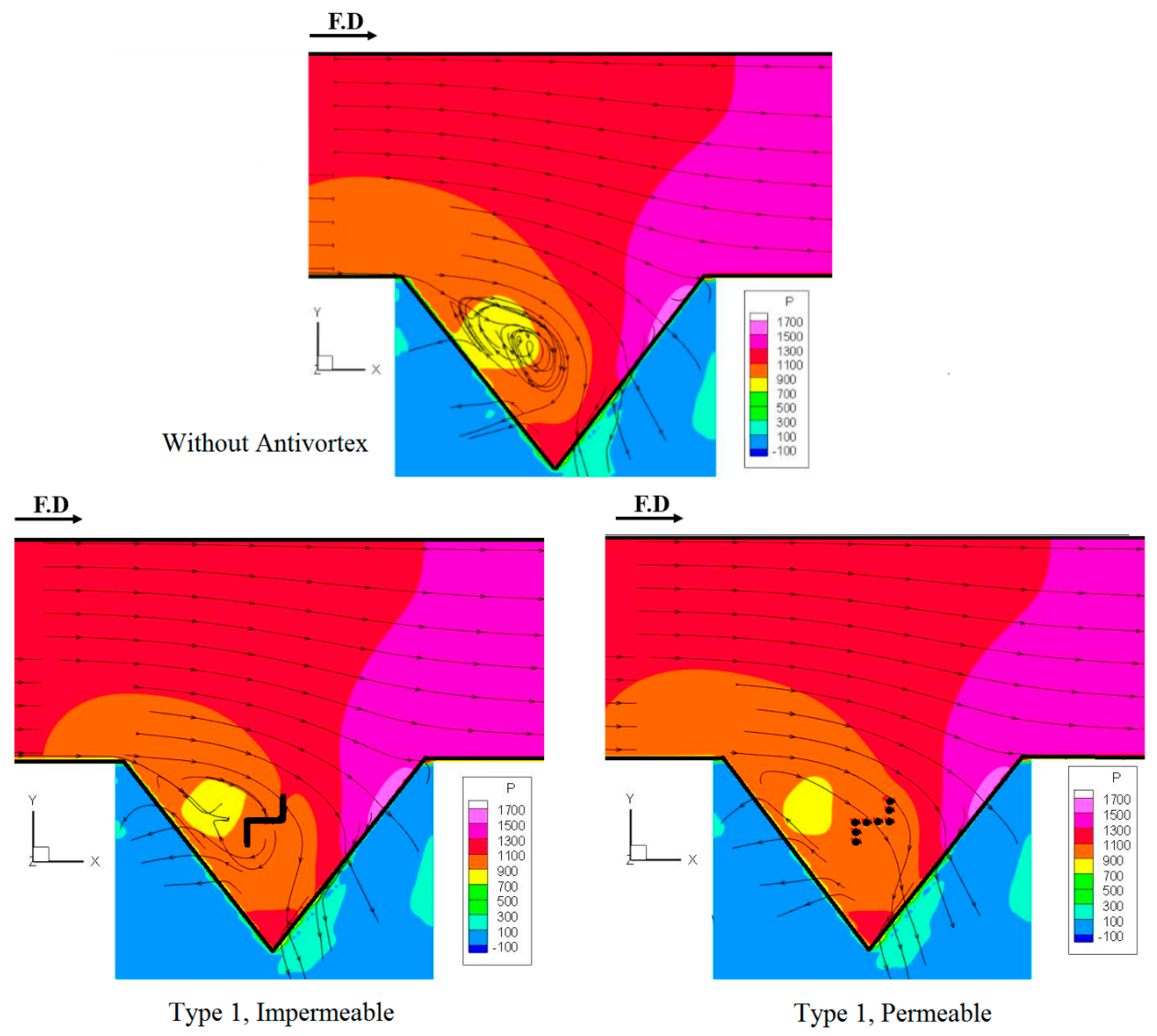
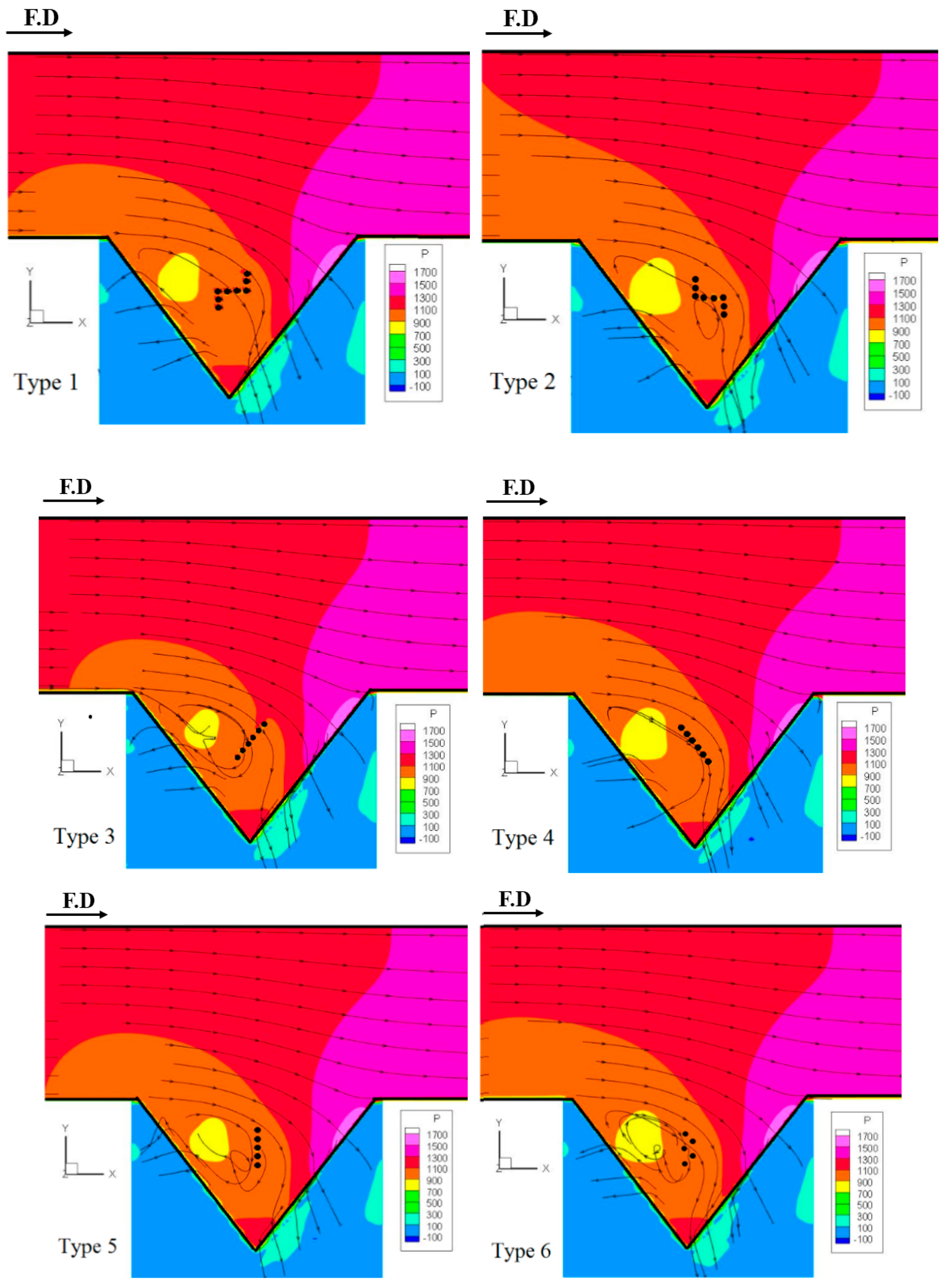
As mentioned earlier, regarding the flow path from the main channel to the side weir, the current entering the side weir causes larger vortexes and increases the pressure in that area. This increase in pressure intensifies the secondary currents, creates vortexes, and reduces the discharge coefficient. Figure 15 shows the cavity of the vortex inside the side weir (yellow zone), created due to the secondary flow, which reduces the hydraulic performance of the weir. The antivortex structure, especially Permeable Antivortex Type 1, reduced the pressure density and the dimensions of the vortex inside the labyrinth side weir, which increased the discharge coefficient of the labyrinth side weirs. Comparing the antivortex shapes indicates that Type 1 outperforms the other antivortexes (see Figure 16).
3.4. The effect of Antivortex Height
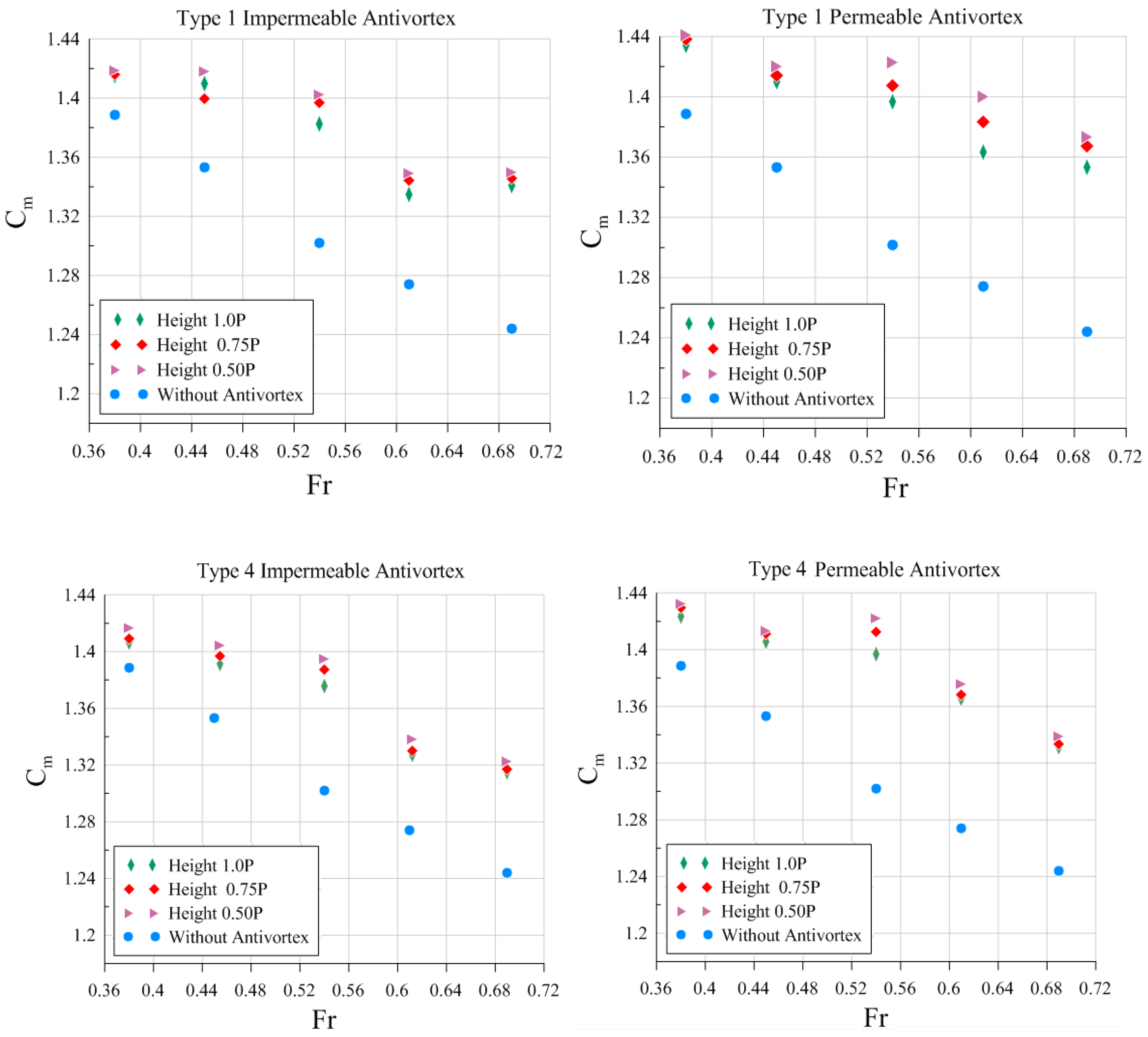
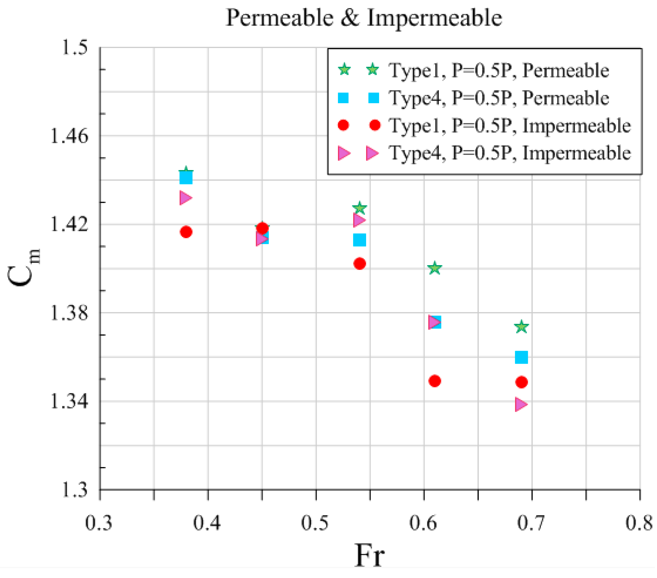
According to the results in this study, Antivortex Types 1 and 4 increase the discharge coefficient more than other types do. Figure 17 shows a comparison of the discharge coefficients of permeable and impermeable antivortexes of Types 1 and 4 with three different antivortex heights. Decreasing the height of the antivortex increases the discharge coefficient to 4.2%. The effect of the height of the antivortex on the discharge coefficient can be explained by the existence of the vortex region near the bottom of the apex of the side weir. This vortex region has a strong secondary motion, and the intensity of this secondary motion decreases as antivortex height decreases.
The discharge coefficients of triangular labyrinth side weirs with an antivortex were found to have higher values than those without an antivortex structure. The discharge over triangular labyrinth side weirs is greater with a permeable antivortex than it is with an impermeable antivortex. In particular, the triangular labyrinth side weirs with a permeable antivortex and P’ = 0.5 P has higher Cm values, so it increased the discharge coefficient by 13.4%. The reason for this increase is that a proper geometric arrangement and height of Antivortex Type 1 reduces the vortexes caused by the secondary flows. The reduction in the intensity of the secondary motion near the bottom of the apex of the side weir and the lower amount of flow blockage over the triangular labyrinth side weir are the main factors contributing to the superior performance of Permeable Antivortex Type 1 with P′= 0.5 P (see Figure 18).
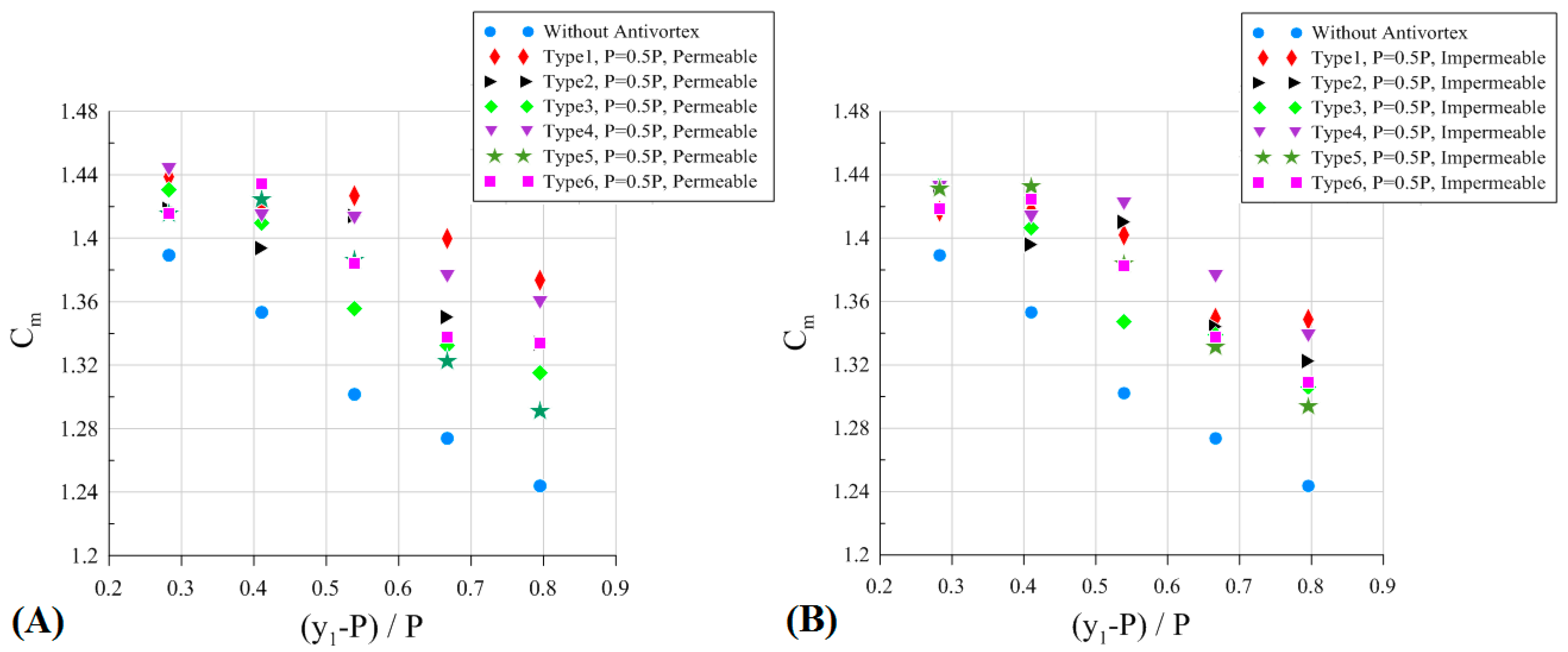
The values of Cm are plotted against (y1 − P)/P in Figure 19. The discharge coefficient decreases as flow depth upstream of the triangular labyrinth side weir increases. Tullis et al. [47] and Emiroglu et al. [18] also reported a similar tendency. In similar flow depths, the use of an antivortex in either a permeable or impermeable state increases the discharge coefficient of the triangular labyrinth side weir.
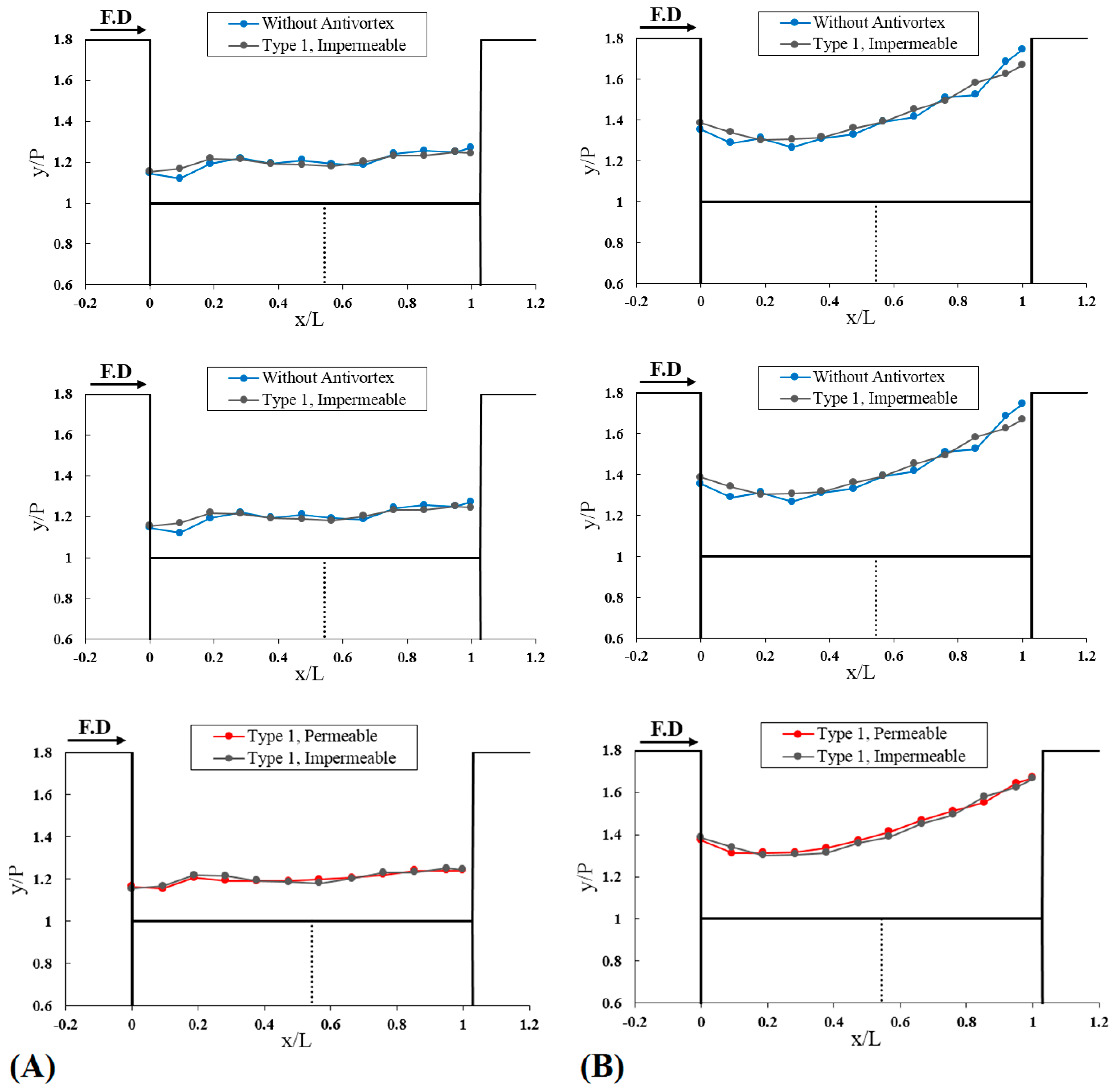
Figure 20 shows the water free surface profile along the crest of the triangular labyrinth side weir for the two types of antivortexes that showed the best performance. The antivortexes reduce the fluctuations of the flow passing over the side. A more uniform water surface on the side weir caused greater efficiency and a more uniform discharge. Permeable antivortexes also better control water fluctuations than impermeable antivortexes do.
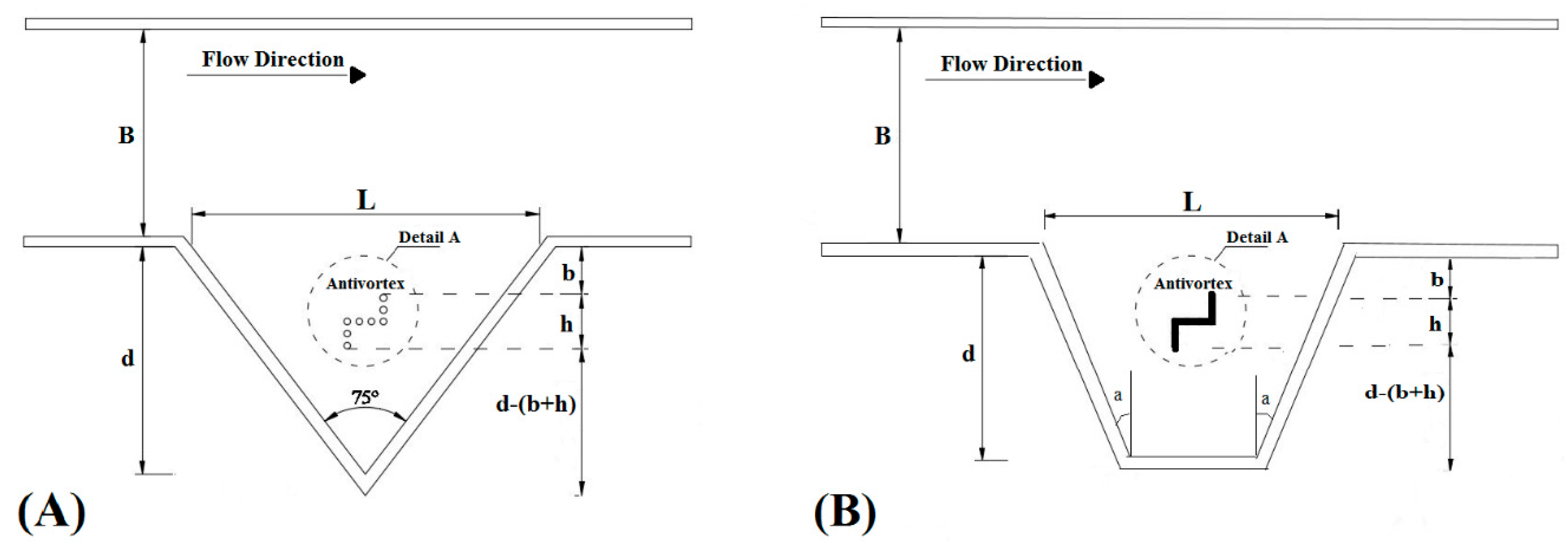
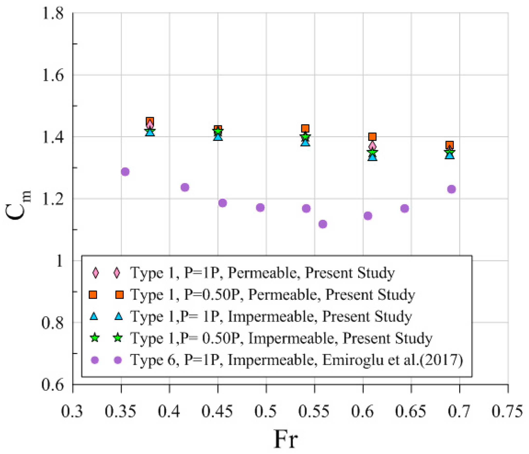
The discharge coefficient values, relative to the triangular labyrinth side weir with the best type of antivortex, were compared with results obtained by Emiroglu et al. [18] on a trapezoidal labyrinth side weir (see Figure 21), as shown in Figure 22. The selected antivortex of the present study (Type 1 with P´ = 1 P and 0.5 P) outperforms the selected antivortex (Type 6) of Emiroglu et al. [18]. The discharge coefficient in the case of using a permeable antivortex with P´ = 0.5 P, compared to the results of Emiroglu et al. [18], is 11% higher. The primary reason for this increase in the discharge coefficient of the triangular labyrinth side weir can be attributed to the permeability and proper height of the antivortex used in this study.
4. Conclusions
The aim of this work is to delineate an optimal configuration of the antivortex, embedded in triangular labyrinth side weirs that maximize the discharge. Numerical investigations were carried out in a straight channel using triangular labyrinth side weirs with six different types of antivortexes embedded inside to observe discharge coefficient behavior. The effect of geometric antivortex parameters, in permeable and impermeable states, on the discharge coefficient in various hydraulic conditions and with different Froude numbers was also evaluated.
The numerical model was first compared with experimental results from the literature to demonstrate the suitability of the calculations to adequately capture flow features. The maximum error of the water free surface profiles between the experimental data and the numerical results for the triangular labyrinth side weir is 3.1%, which confirms the ability of the numerical model to predict specifications of flow over a triangular labyrinth side weir.
The use of antivortexes inside the side weir improves the hydraulic performance of the side weir through a decrease of secondary flow motion intensity and an increase in the discharge coefficient. Moreover, permeable antivortexes have better performance than impermeable ones.
By investigating the effect of antivortex height on the discharge coefficient of the flow over triangular labyrinth side weirs, it was observed that antivortexes with half of the height of the side weir (P´ = 0.5 P) have the best performance than other heights of the side weir and increase the discharge coefficient by 4.2%.
Among the tested antivortex, permeable antivortex Type 1 with 0.5 P height has the best performance at reducing the formation of vortices in the triangular labyrinth side weir and increasing the discharge coefficient up to about 13.4%.
The preliminary results reveal Antivortex 1 as the more efficient to be used in terms of discharge capacity of the side weir. The selected prototype can be applied in river restoration and flood defense studies, optimizing and maximizing the diverted discharge for a given crest length on the plan.
Author Contributions
Conceptualization, A.G., S.F., S.A., and S.D.F.; methodology, A.G., S.F., S.A., and S.D.F.; software, A.G. and S.F.; validation, A.G., S.F., and S.D.F.; formal analysis, A.G., S.F., and S.D.F.; investigation, S.F., S.A., and S.D.F.; writing—original draft preparation, A.G., S.F., S.A., and S.D.F.; writing—review and editing, A.G., S.F., S.A., and S.D.F.; supervision, A.G. and S.A.; project administration, A.G.; funding acquisition, S.D.F. All authors have read and agreed to the published version of the manuscript.
Funding
This research received no external funding.
Informed Consent Statement
Informed consent was obtained from all subjects involved in the study.
Conflicts of Interest
The authors declare no conflict of interest.
References
- De Marchi, G. Essay on the performance of lateral weirs. L’Energia Electerica 1934, 11, 849–860. [Google Scholar]
- Singh, R.; Manivannan, D.; Satyanarayana, T. Discharge coefficient of rectangular side weirs. J. Irrig. Drain. Eng. 1994, 120, 814–819. [Google Scholar] [CrossRef]
- Borghei, M.; Jalili, M.R.; Ghodsian, M. Discharge coefficient for sharp-crested side weir in subcritical flow. J. Hydraul. Eng. 1999, 125, 1051–1056. [Google Scholar] [CrossRef]
- Cosar, A.; Agaccioglu, H. Discharge coefficient of a triangular side-weir located on a curved channel. J. Irrig. Drain. Eng. 2004, 130, 410–423. [Google Scholar] [CrossRef]
- Hyung, P.M.; Sop, R.D. Development of discharge formula for broad crested side weir. J. Korea Water Resour. Assoc. 2010, 43, 525–531. [Google Scholar]
- Muslu, Y. Lateral weir flow model using a curve fitting analysis. J. Hydraul. Eng. 2002, 128, 712–715. [Google Scholar] [CrossRef]
- Rahimpour, M.; Keshavarz, Z.; Ahmadi, M. Flow over trapezoidal side weir. Flow Meas. Instrum. 2011, 22, 507–510. [Google Scholar] [CrossRef]
- Bagheri, S.; Heidarpour, M. Characteristics of flow over rectangular sharp-crested side weirs. J. Irrig. Drain. Eng. 2012, 138, 541–547. [Google Scholar] [CrossRef]
- Ghaderi, A.; Dasineh, M.; Abbasi, S.; Abraham, J. Investigation of trapezoidal sharp-crested side weir discharge coefficients under subcritical flow regimes using CFD. Appl. Water Sci. 2020, 10, 31. [Google Scholar] [CrossRef] [Green Version]
- Venutelli, M. Method of solution of nonuniform flow with the presence of rectangular side weir. J. Irrig. Drain. Eng. 2008, 134, 840–846. [Google Scholar] [CrossRef]
- Emiroglu, M.E.; Kaya, N.; Agaccioglu, H. Discharge capacity of labyrinth side weir located on a straight channel. J. Irrig. Drain. Eng. 2010, 136, 37–46. [Google Scholar] [CrossRef]
- Kabiri-Samani, A.; Borghei, S.M.; Esmaili, H. Hydraulic performance of labyrinth side weirs using vanes or piles. J. Water Manag. ICE 2011, 164, 229–241. [Google Scholar] [CrossRef]
- Khameneh, H.Z.; Khodashenas, S.R.; Esmaili, K. The effect of increasing the number of cycles on the performance of labyrinth side weir. Flow Meas. Instrum. 2014, 39, 35–45. [Google Scholar] [CrossRef]
- Emiroglu, M.E.; Kaya, N. Discharge coefficient for trapezoidal labyrinth side weir in subcritical flow. Water Resour. Manag. 2011, 25, 1037–1058. [Google Scholar] [CrossRef]
- Emiroglu, M.E.; Aydin, M.C.; Kaya, N. Discharge characteristics of a trapezoidal labyrinth side weir with one and two cycles in subcritical flow. J. Irrig. Drain. Eng. 2014, 140, 04014007. [Google Scholar] [CrossRef]
- Nezami, F.; Farsadizadeh, D.; Nekooie, M.A. Discharge coefficient for trapezoidal side weir. Alex. Eng. J. 2015, 54, 595–605. [Google Scholar] [CrossRef] [Green Version]
- Aydin, M.C.; Emiroglu, M.E. Numerical analysis of subcritical flow over two-cycle trapezoidal labyrinth side weir. Flow Meas. Instrum. 2016, 48, 20–28. [Google Scholar] [CrossRef]
- Emiroglu, M.E.; Gogus, M.; Tunc, M.; Islamoglu, K. Effects of Antivortex Structures Installed on Trapezoidal Labyrinth Side Weirs on Discharge Capacity and Scouring. J. Irrig. Drain. Eng. 2017, 143, 04017006. [Google Scholar] [CrossRef]
- Abdollahi, A.; Kabiri-Samani, A.; Asghari, K.; Atoof, H.; Bagheri, S. Numerical modeling of flow field around the labyrinth side-weirs in the presence of guide vanes. ISH J. Hydraul. Eng. 2017, 23, 71–79. [Google Scholar] [CrossRef]
- Aydin, M.C.; Ulu, A.E. Antivortex Effects on Two-Cycle Trapezoidal Labyrinth Side Weirs. J. Irrig. Drain. Eng. 2017, 143, 06017004. [Google Scholar] [CrossRef]
- Karimi, M.; Ghazizadeh, M.R.J.; Saneie, M.; Attari, J. Flow characteristics over asymmetric triangular labyrinth side weirs. Flow Meas. Instrum. 2019, 68, 101574. [Google Scholar] [CrossRef]
- Esmaili, H. Increasing Efficiency of Side Weirs due to the Inlet Geometry. Master’s Thesis, Isfahan University of Technology, Isfahan, Iran, 2009. [Google Scholar]
- Flow Science Inc. FLOW-3D V 11.2 User’s Manual; Flow Science, Inc.: Santa Fe, NM, USA, 2016. [Google Scholar]
- Hirt, C.W.; Nichols, B.D. Volume of fluid (VOF) method for the dynamics of free boundaries. J. Comput. Phys. 1981, 39, 201–225. [Google Scholar] [CrossRef]
- Wilcox, D.C. Turbulence Modeling for CFD, 3rd ed.; DCW Industries, Inc.: La Canada, CA, USA, 2006. [Google Scholar]
- Zhenwei, Z.; Haixia, L. Experimental investigation on the anisotropic tensorial eddy viscosity model for turbulence flow. Int. J. Heat Technol. 2016, 34, 186–190. [Google Scholar]
- Chero, E.; Torabi, M.; Zahabi, H.; Ghafoorisadatieh, A.; Bina, K. Numerical analysis of the circular settling tank. Drink. Water Eng. Sci. 2019, 12, 39–44. [Google Scholar] [CrossRef] [Green Version]
- Zahabi, H.; Torabi, M.; Alamatian, E.; Bahiraei, M.; Goodarzi, M. Effects of Geometry and Hydraulic Characteristics of Shallow Reservoirs on Sediment Entrapment. Water 2018, 10, 1725. [Google Scholar] [CrossRef] [Green Version]
- Sangsefidi, Y.; MacVicar, B.; Ghodsian, M.; Mehraein, M.; Torabi, M.; Savage, B.M. Evaluation of flow characteristics in labyrinth weirs using response surface methodology. Flow Meas. Instrum. 2019, 69, 101617. [Google Scholar] [CrossRef]
- Daneshfaraz, R.; Ghaderi, A.; Akhtari, A.; Di Francesco, S. On the Effect of Block Roughness in Ogee Spillways with Flip Buckets. Fluids 2020, 5, 182. [Google Scholar] [CrossRef]
- Ghaderi, A.; Abbasi, S.; Abraham, J.; Azamathulla, H.M. Efficiency of Trapezoidal Labyrinth Shaped Stepped Spillways. Flow Meas. Instrum. 2020, 72, 101711. [Google Scholar] [CrossRef]
- Ghaderi, A.; Daneshfaraz, R.; Dasineh, M.; Di Francesco, S. Energy Dissipation and Hydraulics of Flow over Trapezoidal–Triangular Labyrinth Weirs. Water 2020, 12, 1992. [Google Scholar] [CrossRef]
- Ansari, U.S.; Patil, L.G. Numerical analysis of triangular labyrinth side weir in triangular channel. ISH J. Hydraul. Eng. 2020, 1–8. [Google Scholar] [CrossRef]
- Pourshahbaz, H.; Abbasi, S.; Pandey, M.; Pu, J.H.; Taghvaei, P.; Tofangdar, N. Morphology and hydrodynamics numerical simulation around groynes. ISH J. Hydraul. Eng. 2020, 1–9. [Google Scholar] [CrossRef]
- Yakhot, V.; Orszag, S.A. Renormalization group analysis of turbulence. I. basic theory. J. Sci. Comput. 1986, 1, 3–51. [Google Scholar] [CrossRef]
- Ghaderi, A.; Daneshfaraz, R.; Abbasi, S.; Abraham, J. Numerical analysis of the hydraulic characteristics of modified labyrinth weirs. Int. J. Energy Water Resour. 2020, 4, 425–436. [Google Scholar] [CrossRef]
- Sosnowski, M. Evaluation of Heat Transfer Performance of a Multi-Disc Sorption Bed Dedicated for Adsorption Cooling Technology. Energies 2019, 12, 4660. [Google Scholar] [CrossRef] [Green Version]
- Ghaderi, A.; Dasineh, M.; Aristodemo, F.; Ghahramanzadeh, A. Characteristics of free and submerged hydraulic jumps over different macroroughnesses. J. Hydroinform. 2020, 22, 1554–1572. [Google Scholar] [CrossRef]
- Daneshfaraz, R.; Minaei, O.; Abraham, J.; Dadashi, S.; Ghaderi, A. 3-D Numerical simulation of water flow over a broad-crested weir with openings. ISH J. Hydraul. Eng. 2019, 1–9. [Google Scholar] [CrossRef]
- Ghaderi, A.; Abbasi, S. CFD simulation of local scouring around airfoil-shaped bridge piers with and without collar. Sādhanā 2019, 4, 216. [Google Scholar] [CrossRef] [Green Version]
- Roache, P.J. Perspective: A Method for Uniform Reporting of Grid Refinement Studies. J. Fluids Eng. 1994, 116, 405–413. [Google Scholar] [CrossRef]
- Celik, I.B.; Ghia, U.; Roache, P.J. Procedure for estimation and reporting of uncertainty due to discretization in CFD applications. J. Fluids Eng. 2020, 130, 078001. [Google Scholar]
- El-Khashab, A.M.M.; Smith, K.V.H. Experimental investigation of flow over side weirs. J. Hydraul. Div. 1976, 102, 1255–1268. [Google Scholar]
- Garcia Perez, M.; Vakkilainen, E.A. Comparison of turbulence models and two and three dimensional meshes for unsteady CFD ash deposition tools. Fuel 2019, 237, 806–811. [Google Scholar] [CrossRef]
- Salim, M.S.; Cheah, S.C. Wall y+ strategy for dealing with wallbounded turbulent flows. In Proceedings of the International Multiconference of Engineers and Computer Scientists IMECS, Hong Kong, 18–20 March 2009; Volume 2. [Google Scholar]
- Gualtieri, C. RANS-based simulation of transverse turbulent mixing in a 2D geometry. Environ. Fluid Mech. 2010, 10, 137–156. [Google Scholar] [CrossRef]
- Tullis, J.P.; Amanian, N.; Waldron, D. Design of labyrinth spillways. J. Hydraul. Eng. 1995, 121, 247–255. [Google Scholar] [CrossRef]
Figure 1.
Schematic view of a triangular labyrinth side weir.

Figure 2.
Geometric characteristics and location of permeable and impermeable antivortexes.


Figure 3.
Applied boundary conditions.

Figure 4.
Gridding for FLOW-3D simulations.

Figure 5.
Comparison of the discharge coefficient obtained from numerical simulation and experimental results.
Figure 5.
Comparison of the discharge coefficient obtained from numerical simulation and experimental results.

Figure 6.
Comparison of the water free surface profile along the crest of the triangular labyrinth side weir (axis A-A) from numerical simulation and experimental results.
Figure 6.
Comparison of the water free surface profile along the crest of the triangular labyrinth side weir (axis A-A) from numerical simulation and experimental results.

Figure 7.
Velocity profiles along the axis (A-A) and (B-B) the main channel, upstream of the triangular labyrinth side weir.
Figure 7.
Velocity profiles along the axis (A-A) and (B-B) the main channel, upstream of the triangular labyrinth side weir.

Figure 8.
Lateral flow along the opening length of the triangular labyrinth side weir: (A) Streamlines; (B) pressure contour.
Figure 8.
Lateral flow along the opening length of the triangular labyrinth side weir: (A) Streamlines; (B) pressure contour.

Figure 9.
Schematic of streamlines and vortexes formed inside the triangular labyrinth side weir, (A) without an antivortex and (B) with an antivortex.
Figure 9.
Schematic of streamlines and vortexes formed inside the triangular labyrinth side weir, (A) without an antivortex and (B) with an antivortex.


Figure 10.
Variations in Cd with Fr in the triangular labyrinth side weir with and without antivortexes.
Figure 10.
Variations in Cd with Fr in the triangular labyrinth side weir with and without antivortexes.

Figure 11.
The secondary flow intensity along of the triangular labyrinth side weir with and without antivortexes.
Figure 11.
The secondary flow intensity along of the triangular labyrinth side weir with and without antivortexes.

Figure 12.
Variations in Cd with P/y1 for the triangular labyrinth side weir with permeable and impermeable antivortexes.
Figure 12.
Variations in Cd with P/y1 for the triangular labyrinth side weir with permeable and impermeable antivortexes.

Figure 13.
Longitudinal velocity contours in the main channel and around the antivortex structure.

Figure 14.
Longitudinal velocity contours near the surface and around the different antivortex structures.
Figure 14.
Longitudinal velocity contours near the surface and around the different antivortex structures.


Figure 15.
Comparison of pressure over the side weir with an antivortex structure.

Figure 16.
Pressure over the side weir and around the different antivortex structures.

Figure 17.
The effect of the antivortex height on the discharge coefficient of the triangular labyrinth side weir.
Figure 17.
The effect of the antivortex height on the discharge coefficient of the triangular labyrinth side weir.

Figure 18.
Performance of Permeable and Impermeable Antivortex Types 1 and 4 with a height of 0.5 P.
Figure 18.
Performance of Permeable and Impermeable Antivortex Types 1 and 4 with a height of 0.5 P.

Figure 19.
Variations in Cm with (y1 − P)/P in triangular labyrinth side weirs. (A): Permeable antivortex; (B): Impermeable antivortex.
Figure 19.
Variations in Cm with (y1 − P)/P in triangular labyrinth side weirs. (A): Permeable antivortex; (B): Impermeable antivortex.

Figure 20.
Free surface profile along the crest of the triangular labyrinth side weir with antivortexes. (A) Fr = 0.38; (B) Fr = 0.69.
Figure 20.
Free surface profile along the crest of the triangular labyrinth side weir with antivortexes. (A) Fr = 0.38; (B) Fr = 0.69.

Figure 21.
View of the best model of the antivortex inside the labyrinth side weir. (A): Present study; (B): Emiroglu et al. [18].
Figure 21.
View of the best model of the antivortex inside the labyrinth side weir. (A): Present study; (B): Emiroglu et al. [18].

Figure 22.
Comparison of antivortexes in the present study with antivortexes used by Emiroglu et al. [18] in terms of discharge coefficient values.
Figure 22.
Comparison of antivortexes in the present study with antivortexes used by Emiroglu et al. [18] in terms of discharge coefficient values.


Table 1.
Geometric characteristics of the triangular labyrinth side weir from Esmalili [22] and Kabiri Samani et al. [12].
| Models | y1 (m) | B (m) | L (m) | P (m) | |
|---|---|---|---|---|---|
| Numerical and Physical Models | 0.18 | 0.4 | 75 | 0.525 | 0.156 |
Table 2.
Geometrical properties of antivortex models and hydraulic flow parameters.
| Variable | Range |
|---|---|
| Channel width (B_ m) | 0, 50 |
| Side weir opening length (L_ m) | 0.525 |
| Side weir height (P_ m) | 0.156 |
| Side weir depth (d_ m) | 0.34 |
| Antivortex length in the side weir (h_ m) | 0.081 |
| Antivortex height (P’_ m) | 0.078, 0.117, 0.156 |
| The antivortex distance from the beginning of the weir (b_ m) | 0.072 |
| Diameter of the permeable antivortex bars (Ø_ m) | 0.01 |
| Permeability (r_ %) | 0, 50 |
| Upstream Froude number (F_-) | 0.38–0.69 |
| Upstream depth of flow (y0_m) | 0.195–0.28 |
Table 3.
Characteristics of the meshes tested in the convergence analysis.
| Mesh | Nested Block Cell Size | Containing Block Cell Size |
|---|---|---|
| 1 | 1 cm | 1.65 cm |
| 2 | 0.75 cm | 1.31 cm |
| 3 | 0.60 cm | 1.20 cm |
Table 4.
GCI (grid convergence index) calculation.
| Mesh (cm) | N (-) | r (-) | p (-) | E (%) | GCI (%) |
|---|---|---|---|---|---|
| 0.60 | 804,112 | 1.25 | 2.72 | 2.59 | 3.87 |
| 0.75 | 568,062 | 1.33 | |||
| 1.00 | 316,869 | - |
Table 5.
Grid details in the numerical domain.
| Block | Max Cell Size (cm) | Min Cell Size (cm) | Near Wall Distance (cm) | Range of Dimensionless Distance y+ |
|---|---|---|---|---|
| Containing and nested block | 1.31 × 1.31 × 1.31 | 0.75 × 0.75 × 0.75 | 0.55 | 54 < y+ < 79 |
Publisher’s Note: MDPI stays neutral with regard to jurisdictional claims in published maps and institutional affiliations. |
© 2020 by the authors. Licensee MDPI, Basel, Switzerland. This article is an open access article distributed under the terms and conditions of the Creative Commons Attribution (CC BY) license (http://creativecommons.org/licenses/by/4.0/).
Share and Cite
MDPI and ACS Style
Abbasi, S.; Fatemi, S.; Ghaderi, A.; Di Francesco, S. The Effect of Geometric Parameters of the Antivortex on a Triangular Labyrinth Side Weir. Water 2021, 13, 14. https://0-doi-org.brum.beds.ac.uk/10.3390/w13010014
AMA Style
Abbasi S, Fatemi S, Ghaderi A, Di Francesco S. The Effect of Geometric Parameters of the Antivortex on a Triangular Labyrinth Side Weir. Water. 2021; 13(1):14. https://0-doi-org.brum.beds.ac.uk/10.3390/w13010014
Chicago/Turabian StyleAbbasi, Saeed, Sajjad Fatemi, Amir Ghaderi, and Silvia Di Francesco. 2021. "The Effect of Geometric Parameters of the Antivortex on a Triangular Labyrinth Side Weir" Water 13, no. 1: 14. https://0-doi-org.brum.beds.ac.uk/10.3390/w13010014
Note that from the first issue of 2016, this journal uses article numbers instead of page numbers. See further details here.