Variable Coefficient Exact Solutions for Some Nonlinear Conformable Partial Differential Equations Using an Auxiliary Equation Method

Abstract

The objective of this present paper is to utilize an auxiliary equation method for constructing exact solutions associated with variable coefficient function forms for certain nonlinear partial differential equations (NPDEs) in the sense of the conformable derivative. Utilizing the specific fractional transformations, the conformable derivatives appearing in the original equation can be converted into integer order derivatives with respect to new variables. As for applications of the method, we particularly obtain variable coefficient exact solutions for the conformable time (2 + 1)-dimensional Kadomtsev–Petviashvili equation and the conformable space-time (2 + 1)-dimensional Boussinesq equation. As a result, the obtained exact solutions for the equations are solitary wave solutions including a soliton solitary wave solution and a bell-shaped solitary wave solution. The advantage of the used method beyond other existing methods is that it provides variable coefficient exact solutions covering constant coefficient ones. In consequence, the auxiliary equation method based on setting all coefficients of an exact solution as variable function forms can be more extensively used, straightforward and trustworthy for solving the conformable NPDEs.

1. Introduction

Over the last few decades, many researchers have thoroughly investigated many methods for finding exact solutions of nonlinear partial differential equations (NPDEs). This is because the exact solutions play a crucial role in exactly describing physical phenomena such as nonlinear wave spreads in incompressible fluid, electromagnetic field, shallow water waves, epidemic diseases and water pollutant modeled by certain NPDEs [1,2,3,4,5]. Precise behaviors of a mathematical system expressed by NPDEs can be analyzed through their exact solutions. In addition, symbolic computer software packages (e.g., Mathematica and Maple) have been continuously and progressively developed for several years. According to these reasons, it brings a vital challenge for solving NPDEs to scholars’ attention. Scientists and researchers have attempted to propose new and efficient techniques for constructing exact traveling wave solutions of NPDEs such as the $(G^{\prime }/G,1/G)$-expansion method [6,7,8], the multiple Exp-function method [9], the modified Jacobi elliptic expansion method [10], the improved Riccati equation mapping method [11] and the modified extended simple equation [12].

This paper addresses the use of an auxiliary equation method used to generate variable coefficient exact solutions for a particular type of NPDEs. Hence, some significant investigations of the method and its modifications are briefly reviewed as follows. Pinar [13] used appropriate Lie group transformations and the auxiliary equation method in which the Bernoulli differential equation is considered to find exact solutions of the foam-drainage equation. Mahak and Akram [14] utilized the modified auxiliary equation method to construct bright soliton waves, stable bright periodic waves and symmetric waves, which were exact solutions of the perturbed nonlinear Schrödinger equation with Kerr law nonlinearity. The modified form of the auxiliary equation method was employed to determine a large family of optical solutions to the Kundu–Eckhaus equation [15]. Moreover, the auxiliary equation method was applied to obtain exact traveling wave solutions of (2 + 1)-dimensional Zoomeron equation with conformable time derivative and the third order modified KdV equation with conformable time derivative [16]. The solutions obtained by the method were expressed in terms of the exponential function. More applications of an auxiliary equation method and its improvements can be found in [17,18,19,20,21,22] and the references therein.

In this work, we utilized an auxiliary equation method to extract exact solutions of two nonlinear conformable partial differential equations in which the conformable partial derivatives are involved. The two equations are described as follows.

• The conformable time (2 + 1)-dimensional Kadomtsev–Petviashvili equation of order $0<\alpha \le 1$ is given as

  $$\frac{\partial }{\partial x}\left(\frac{{\partial }^{\alpha }u}{\partial t^{\alpha }}+6u\frac{\partial u}{\partial x}+\frac{{\partial }^{3}u}{\partial x^3}\right)-\mu \frac{{\partial }^{2}u}{\partial y^2}=0,$$

  (1)

  where $\frac{{\partial }^{\alpha }u}{\partial t^{\alpha }}$ is the conformable partial derivative of the dependent variable $u=u\left(x,y,t\right)$ with respect to the independent variable t of order $\alpha$ and $\mu$ is a positive real number. If $\alpha =1,$ Equation (1) becomes the integer order (2 + 1)-dimensional Kadomtsev–Petviashvili equation [23,24,25] describing the evolution of nonlinear, long waves of small amplitudes with slow dependence on the transverse coordinate. In physics, this equation often provides multi-soliton solutions.
• The conformable space-time (2 + 1)-dimensional Boussinesq equation is

  $$\frac{{\partial }^{2\alpha }u}{\partial t^{2\alpha }}-\frac{{\partial }^{2\alpha }u}{\partial x^{2\alpha }}-\frac{{\partial }^{2\alpha }u}{\partial y^{2\alpha }}-\frac{{\partial }^{2\alpha }{u}^2}{\partial x^{2\alpha }}-\frac{{\partial }^{4\alpha }u}{\partial x^{4\alpha }}=0,0<\alpha \le 1.$$

  (2)
  All of the partial derivatives appearing in Equation (2) are the conformable partial derivatives. When $\alpha =1,$ Equation (2) turns out to be the integer order (2 + 1)-dimensional Boussinesq equation [26,27]. The equation describes the propagation of gravity waves on the surface of water, especially the head-on collision of oblique waves.

The arrangement of the rest of this article is organized as follows. In Section 2, the definition of the conformable derivative and its important properties are given. In Section 3, the algorithm of an auxiliary equation method is briefly described. The applications of the method for finding exact solutions of Equations (1) and (2) are demonstrated in Section 4. Also, graphs of the selected exact solutions for the problems are depicted in this section. In Section 5, we present some discussions and conclusions.

2. Conformable Derivative and Its Characteristics

In this section, a definition of the conformable derivative and its essential properties are reviewed as follows.

Definition 1.

Given a function $f:[0,\infty )\to \mathbb{R}$. Then the conformable derivative of f of order α is defined by [28,29,30,31,32,33,34]

$$\begin{array}{c}\hfill D_t^{\alpha }f\left(t\right)=\underset{\epsilon \to 0}{lim}{\displaystyle \frac{f(t+\epsilon t^{1-\alpha })-f\left(t\right)}{\epsilon }},\end{array}$$

(3)

for all $t>0$ and $0<\alpha \le 1.$ If the limit in Equation (3) exists, then one can say that f is α-conformable differentiable at a point $t>0$.

Theorem 1

([28,29,30,31,32,33,34]). Let $\alpha \in (0,1]$, and $f,g$ be α-conformable differentiable at a point $t>0$. Then, we have

$$\begin{array}{ccc}\hfill D_t^{\alpha }\left(\lambda \right)& =& 0,where\lambda =constant,\hfill \\ \hfill D_t^{\alpha }\left(t^{\mu }\right)& =& \mu t^{\mu -\alpha },forall\mu \in \mathbb{R},\hfill \\ \hfill D_t^{\alpha }(af\left(t\right)+bg\left(t\right))& =& a{D}_t^{\alpha }f\left(t\right)+b{D}_t^{\alpha }g\left(t\right),foralla,b\in \mathbb{R},\hfill \\ \hfill D_t^{\alpha }\left(f\left(t\right)g\left(t\right)\right)& =& f\left(t\right)D_t^{\alpha }g\left(t\right)+g\left(t\right)D_t^{\alpha }f\left(t\right),\hfill \\ \hfill D_t^{\alpha }\left({\displaystyle \frac{f\left(t\right)}{g\left(t\right)}}\right)& =& {\displaystyle \frac{g\left(t\right)D_t^{\alpha }f\left(t\right)-f\left(t\right)D_t^{\alpha }g\left(t\right)}{g{\left(t\right)}^2}}.\hfill \end{array}$$

Remark 1.

The conformable derivatives of some interesting functions are as follows [28,29,30,31,32,33,34].

(1) 

$D_t^{\alpha }\left(e^{ct}\right)=c{t}^{1-\alpha }{e}^{ct},$$c\in \mathbb{R}$.

(2) 

$D_t^{\alpha }(sinbt)=b{t}^{1-\alpha }cosbt,b\in \mathbb{R}$.

(3) 

$D_t^{\alpha }(cosbt)=-b{t}^{1-\alpha }sinbt,b\in \mathbb{R}$.

(4) 

$D_t^{\alpha }\left(\frac{1}{\alpha }{t}^{\alpha }\right)=1$.

(5) 

$D_t^{\alpha }\left(f\left(t\right)\right)=t^{1-\alpha }{\displaystyle \frac{df\left(t\right)}{dt}}$, provided that $f\left(t\right)$ is differentiable.

The following chain rule may be useful for a transformation between the conformable derivative and the classical derivative.

Theorem 2

([28,29,30,31,32,33,34]). Let $f:(0,\infty )\to \mathbb{R}$ be a function such that f is differentiable and α-conformable differentiable. Further assume that g is a differentiable function defined in the range of f. Then, we have

$$D_t^{\alpha }(f\circ g)\left(t\right)=t^{1-\alpha }{f}^{\prime }\left(g\left(t\right)\right)g^{\prime }\left(t\right),$$

where the prime symbol ${(}^{\prime })$ represents the ordinary derivative.

3. Algorithm of the Auxiliary Equation Method

In this section, the description of the auxiliary equation method for solving nonlinear partial differential equations, where the associated partial derivatives are the conformable derivative, is provided. Consider a conformable space–time partial differential equation in the independent variables $t,x_1,x_2,\dots ,x_n$ as follows

$$P(u,u_t,u_{x_1},\dots ,u_{x_i},\dots ,u_{x_n},\frac{{\partial }^{\alpha }u}{\partial t^{\alpha }},\frac{{\partial }^{{\beta }_1}u}{\partial x_1^{{\beta }_1}},\dots ,\frac{{\partial }^{{\beta }_i}u}{\partial x_i^{{\beta }_i}},\dots )=0,$$

(4)

where $u=u\left(x_1,\dots ,x_i,\dots ,x_n,t\right)$ is an unknown function and each value of the fractional orders $\alpha ,{\beta }_1,\dots ,{\beta }_n$ and the others appearing in Equation (4) is in $(0,1]$. Here, the symbol $\frac{{\partial }^{\eta }u}{\partial v^{\eta }}$ represents the conformable partial derivative of a dependent variable u with respect to an independent variable v of order $\eta$. Hence, the symbols $\frac{{\partial }^{\alpha }u}{\partial t^{\alpha }},\frac{{\partial }^{{\beta }_1}u}{\partial x_1^{{\beta }_1}}$ and $\frac{{\partial }^{{\beta }_i}u}{\partial x_i^{{\beta }_i}}$, for example, in Equation (4) are the conformable derivatives of the variable u with respect to the variable t of order $\alpha$, to the variable $x_1$ of order ${\beta }_1$ and to the variable $x_i$ of order ${\beta }_i,$ respectively. In addition, the notation P in the equation represents a polynomial of the unknown function u and its various partial derivatives including the conformable derivatives.

Without loss of generality, we may assume that the conformable partial derivatives emerging in Equation (4) are related to only the variables t and $x_i$; however, the other partial derivatives with respect to the remaining variables are of integer orders. Next, the main steps of the auxiliary equation method for solving Equation (4) are described as follows [18].

Step 1: The conformable partial derivatives in Equation (4), which are now $\frac{{\partial }^{\alpha }u}{\partial t^{\alpha }},\frac{{\partial }^{{\beta }_i}u}{\partial x_i^{{\beta }_i}},$ can be converted into integer order partial derivatives with respect to the new variables using the following two fractional complex transformations:

$$\begin{array}{c}\hfill T=c\left(\frac{t^{\alpha }}{\alpha }\right),X_i=k\left(\frac{x_i^{{\beta }_i}}{{\beta }_i}\right),u\left(x_1,\dots ,x_i,\dots ,x_n,t\right)=\tilde{u}\left(x_1,\dots ,X_i,\dots ,x_n,T\right).\end{array}$$

(5)

Using Theorem 2, one can obtain

$$\begin{array}{c}\hfill \begin{array}{cc}\hfill \frac{{\partial }^{\alpha }u}{\partial t^{\alpha }}& =\frac{\partial \tilde{u}}{\partial T}\frac{{\partial }^{\alpha }T}{\partial t^{\alpha }}=c\frac{\partial \tilde{u}}{\partial T}=c{\tilde{u}}_T,\hfill \\ \hfill \frac{{\partial }^{{\beta }_i}u}{\partial x_i^{{\beta }_i}}& =\frac{\partial \tilde{u}}{\partial X_i}\frac{{\partial }^{{\beta }_i}{X}_i}{\partial x_i^{{\beta }_i}}=k\frac{\partial \tilde{u}}{\partial X_i}=k{\tilde{u}}_{X_i}.\hfill \end{array}\end{array}$$

(6)

Consequently, the conformable partial differential Equation (4) can be transformed into an integer order partial differential equation as

$$\tilde{P}\left(\tilde{u},{\tilde{u}}_T,{\tilde{u}}_{x_1},\dots ,{\tilde{u}}_{X_i},\dots ,{\tilde{u}}_{x_n},\dots \right)=0.$$

(7)

Step 2: Assume that the solution of Equation (7) can be written by a polynomial in $\frac{{\psi }^{\prime }\left(\xi \right)}{\psi \left(\xi \right)}$ as

$$\begin{array}{c}\hfill \tilde{u}\left(x_1,\dots ,X_i,\dots ,x_n,T\right)=\sum _{k=0}^m{a}_k\left(x_1,\dots ,X_i,\dots ,x_n,T\right){\left(\frac{{\psi }^{\prime }\left(\xi \right)}{\psi \left(\xi \right)}\right)}^k,\end{array}$$

(8)

where $\xi =\xi \left(x_1,\dots ,X_i,\dots ,x_n,T\right),a_m\left(x_1,\dots ,X_i,\dots ,x_n,T\right)\ne 0,a_{m-1}\left(x_1,\dots ,X_i,\dots ,x_n,T\right),$ $\dots ,a_0\left(x_1,\dots ,X_i,\dots ,x_n,T\right)$ are unknown functions to be determined at a later step and the function $\psi =\psi \left(\xi \right)$ satisfies some certain auxiliary equation expressed in the form

$$\begin{array}{c}\hfill F\left(\psi ,{\psi }^{\prime },{\psi }^{″},\dots \right)=0,\end{array}$$

(9)

for which its solutions are already known. Moreover, the positive integer m in Equation (8) can be computed via the homogeneous balance principle, balancing the degrees between the highest order derivatives and the nonlinear terms occurring in Equation (7). The formulas for computing the degree of some particular terms for this step can be found in Equation (10) of [33].

In particular, one can select the Riccati equation

$${\psi }^{\prime }\left(\xi \right)+\lambda \psi \left(\xi \right)={\psi }^2\left(\xi \right),$$

(10)

where $\lambda \ne 0$ as the auxiliary equation. It is not difficult to verify that

$$\psi \left(\xi \right)=\frac{\lambda }{1+d\lambda e^{\lambda \xi }},$$

(11)

where d is an arbitrary constant, is a solution of Equation (10). Then, we have

$$\frac{{\psi }^{\prime }\left(\xi \right)}{\psi \left(\xi \right)}=-\frac{d{\lambda }^2{e}^{\lambda \xi }}{1+d\lambda e^{\lambda \xi }}.$$

(12)

Specifically choosing $d=\frac{1}{\lambda }$, we obtain

$$\frac{{\psi }^{\prime }\left(\xi \right)}{\psi \left(\xi \right)}=-\frac{\lambda }{2}\left(1+\tanh \left(\frac{\lambda \xi }{2}\right)\right).$$

(13)

Step 3: Substituting Equation (8) into Equation (7) along with the relation between ${\psi }^{\prime }\left(\xi \right)$ and $\psi \left(\xi \right)$ obtained by Equation (9) (or, particularly Equation (10)), and then collecting all terms with the same power of $\psi \left(\xi \right)$ together, the left-hand side of Equation (7) becomes another polynomial in $\psi \left(\xi \right)$. Equating each coefficient of the resulting polynomial to zero, one gives a set of partial differential equations for $\xi \left(x_1,\dots ,X_i,\dots ,x_n,T\right),$ $a_m\left(x_1,\dots ,X_i,\dots ,x_n,T\right),$ $a_{m-1}\left(x_1,\dots ,X_i,\dots ,x_n,T\right),\dots ,$ $a_0\left(x_1,\dots ,X_i,\dots ,x_n,T\right).$

Step 4: Solving the system of the partial differential equations obtained in Step 3 with the help of Maple and using the solutions of Equation (9) (or, particularly the solution in (11)), together with the fractional complex transformations in (5), we eventually obtain exact solutions of Equation (4).

Remark 2.

The idea of setting the solution in (8) in which ξ is a general function of the independent variables including T and $X_i$ in (5) and $\psi \left(\xi \right)$ satisfies the auxiliary Equation (9) is reminiscent of the direct approach called a similarity reduction [35,36]. This method is more general than our technique because it does not specify the auxiliary equation for $\psi \left(\xi \right)$ and involve with group theoretical techniques. In general, the appropriate similarity reduction can reduce the partial differential equation to an ordinary differential equation.

Remark 3.

We can change the solution form (8) and the Riccati equation (10) in the above process so that the new algorithm, called the modified auxiliary equation method, is obtained. To further grasp the modified approaches, we can refer to [13,14,15,20,21]. Some of the alternative auxiliary equations used in the the modified auxiliary equation methods are as follows. The first example is the Bernoulli type differential equation expressed as [13,20]

$${\psi }^{\prime }\left(\xi \right)=P\left(\xi \right)\psi \left(\xi \right)+Q\left(\xi \right){\psi }^k\left(\xi \right),$$

(14)

where $P\left(\xi \right)$ and $Q\left(\xi \right)$ are any functions and $k>1$ is an integer. The solutions of (14) alter depending upon $P\left(\xi \right)$ and $Q\left(\xi \right)$. The second example of the auxiliary equation is [14,15]

$${\psi }^{\prime }\left(\xi \right)=\frac{\beta +\alpha K^{-\psi \left(\xi \right)}+\sigma K^{\psi \left(\xi \right)}}{ln\left(K\right)},$$

(15)

where $\beta ,\alpha$ and σ are parameters to be determined and $K>0,K\ne 1$. The solutions of (15) can be expressed in terms of tangent, cotangent, hyperbolic tangent, hyperbolic cotangent, or rational functions.

4. Applications of the Method

In this section, we applied the auxiliary equation method to construct exact solutions with variable coefficient function forms for the conformable time (2 + 1)-dimensional Kadomtsev–Petviashvili equation and the conformable space–time (2 + 1)-dimensional Boussinesq equation. In addition, some selected solutions obtained using the method are graphically displayed to demonstrate their physical behaviors.

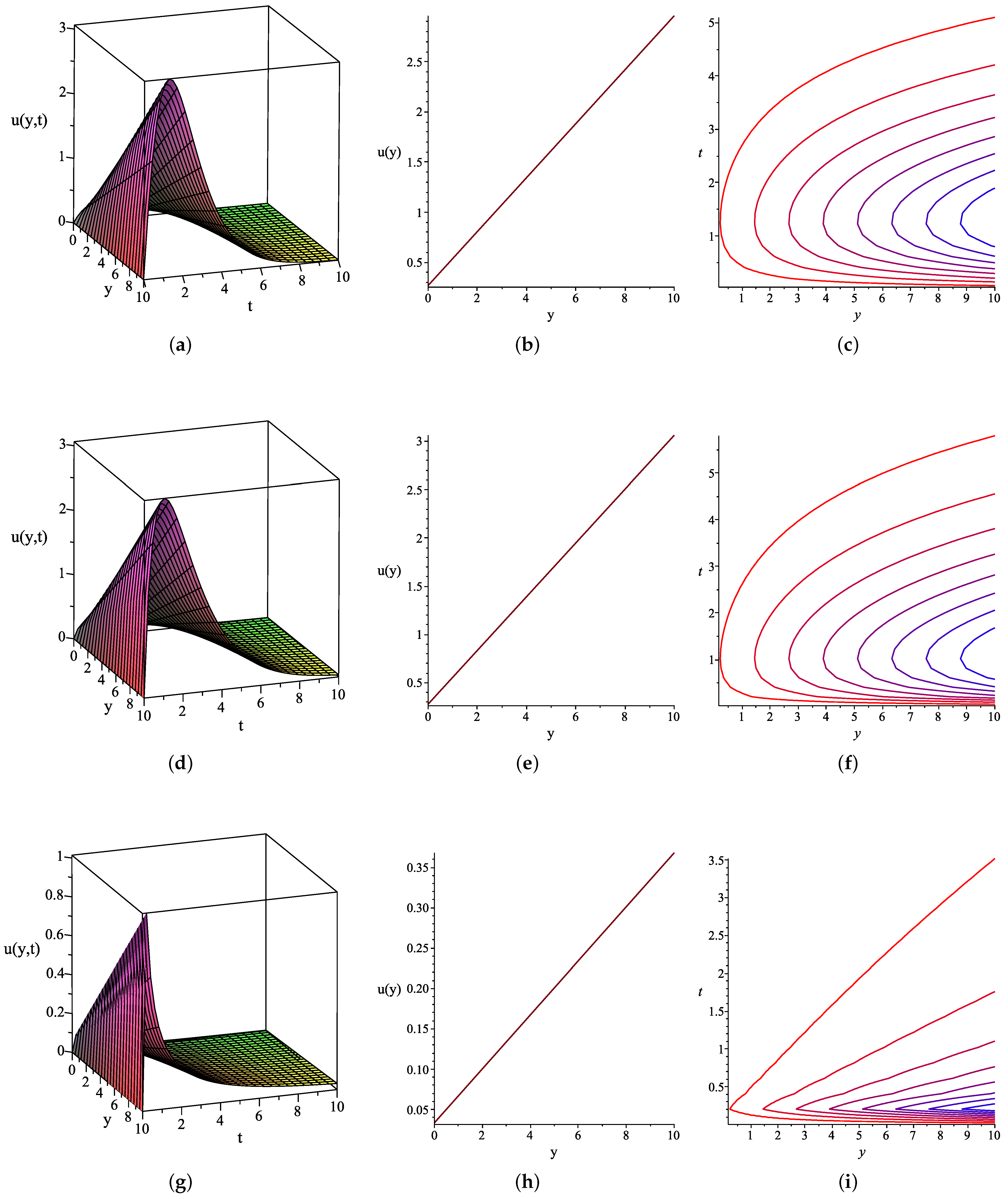
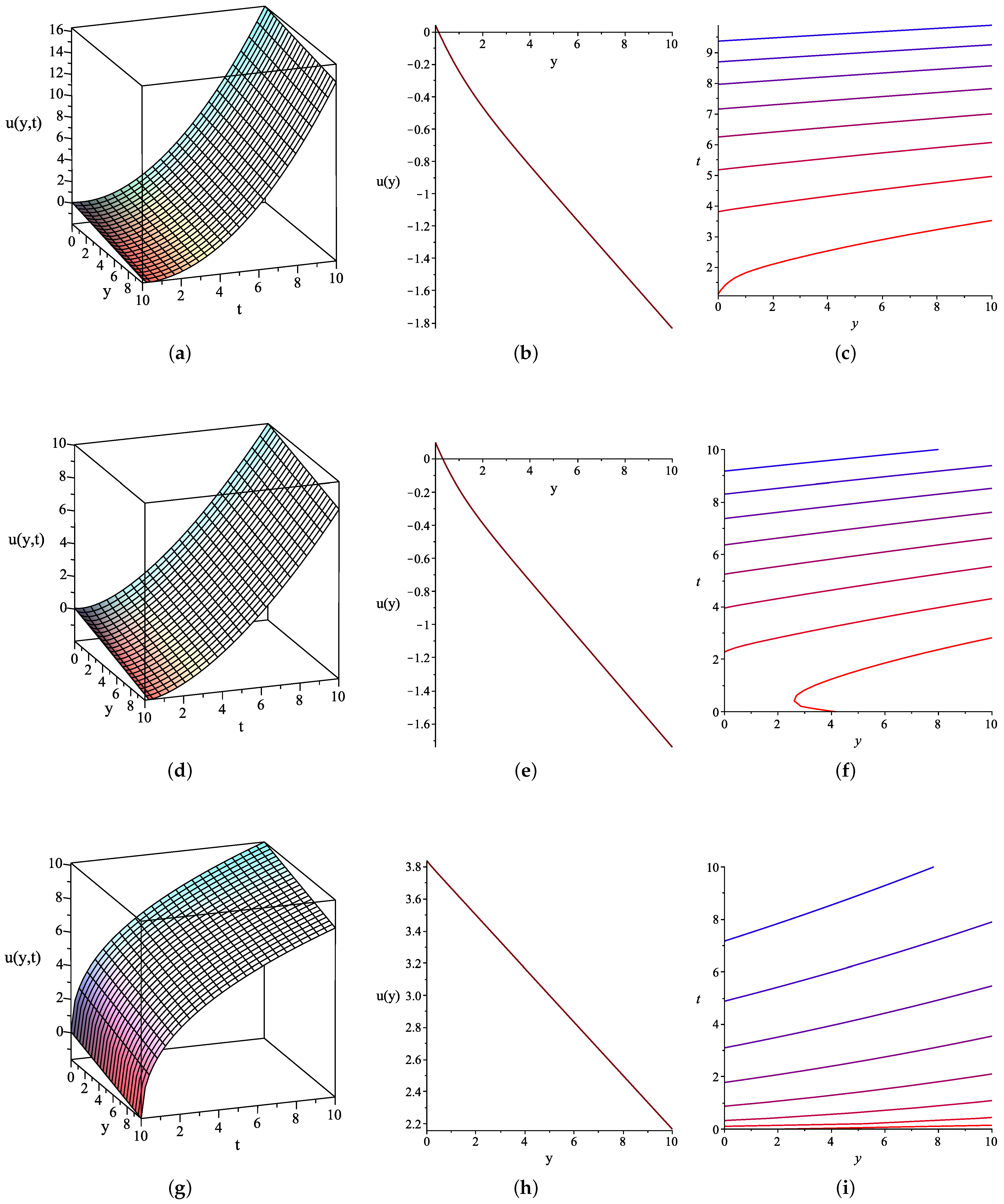
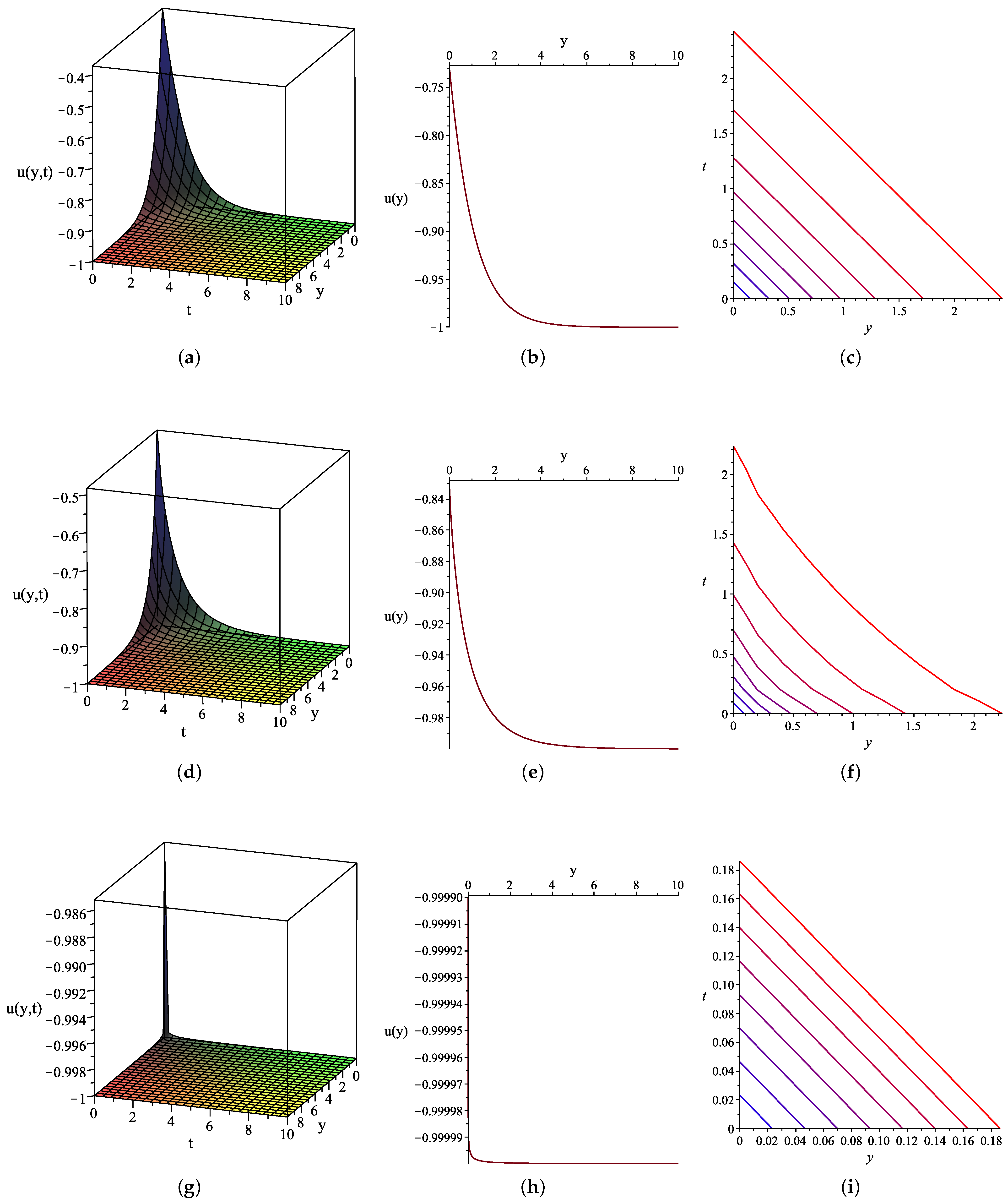
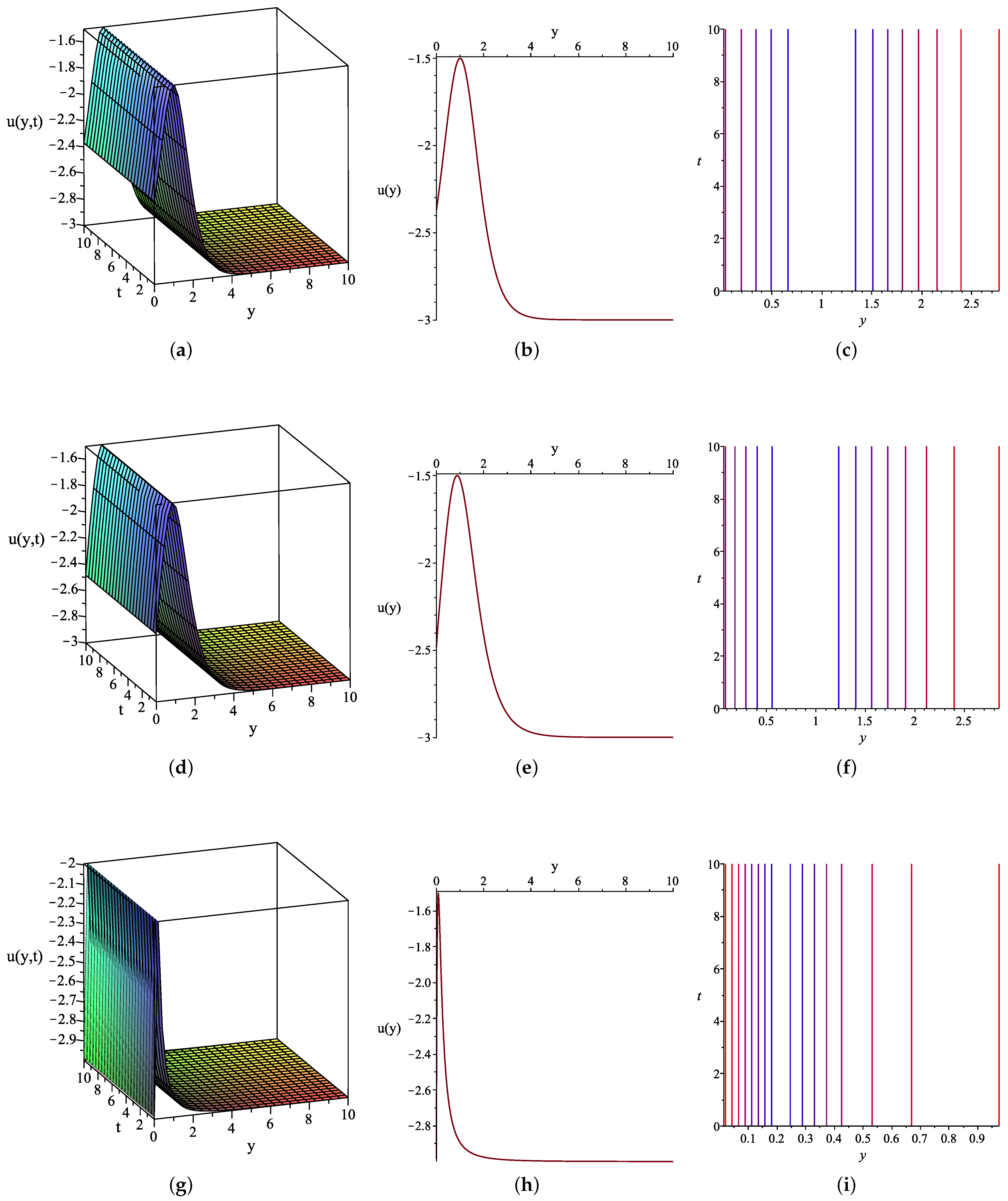
4.1. Conformable Time (2 + 1)-Dimensional Kadomtsev–Petviashvili Equation

We revisit the conformable time (2 + 1)-Kadomtsev–Petviashvili equation expressed as

$$\frac{\partial }{\partial x}\left(\frac{{\partial }^{\alpha }u}{\partial t^{\alpha }}+6u\frac{\partial u}{\partial x}+\frac{{\partial }^{3}u}{\partial x^3}\right)-\mu \frac{{\partial }^{2}u}{\partial y^2}=0,0<\alpha \le 1,$$

(16)

where $\frac{{\partial }^{\alpha }u}{\partial t^{\alpha }}$ is the conformable partial derivative of the dependent variable $u=u\left(x,y,t\right)$ with respect to the independent variable t of order $\alpha$ and $\mu$ is a positive real number. Applying the transformations for the variable t and u as

$$T=c\left(\frac{t^{\alpha }}{\alpha }\right),u\left(x,y,t\right)=\tilde{u}\left(x,y,T\right),$$

(17)

where c is an arbitrary constant and using the chain rule in Theorem 2, we then have $\frac{{\partial }^{\alpha }u}{\partial t^{\alpha }}=\frac{\partial \tilde{u}}{\partial T}\frac{{\partial }^{\alpha }T}{\partial t^{\alpha }}=c\frac{\partial \tilde{u}}{\partial T}=c{\tilde{u}}_T$. Performing a small algebraic manipulation, Equation (16) is reduced into the following integer order partial differential equation

$$c{\tilde{u}}_{Tx}+6{\left({\tilde{u}}_x\right)}^2+6\tilde{u}{\tilde{u}}_{xx}+{\tilde{u}}_{xxxx}-\mu {\tilde{u}}_{yy}=0.$$

(18)

We assume that the solution of Equation (18) can be expressed by a polynomial in $\frac{{\psi }^{\prime }\left(\xi \right)}{\psi \left(\xi \right)}$ as

$$\begin{array}{c}\hfill \tilde{u}\left(x,y,T\right)=\sum _{i=0}^m{a}_i\left(y,T\right){\left(\frac{{\psi }^{\prime }\left(\xi \right)}{\psi \left(\xi \right)}\right)}^i,\end{array}$$

(19)

where $\xi =\xi \left(x,y,T\right)$ and $a_i\left(y,T\right),i=0,1,\dots ,m$ are undetermined functions. For convenience, we here set all coefficients $a_i(i=1,\dots ,m)$ to be functions of only two variables y and T. The function $\psi \left(\xi \right)$, which is the solution of the following auxiliary equation

$${\psi }^{\prime }\left(\xi \right)+\lambda \psi \left(\xi \right)={\psi }^2\left(\xi \right),$$

(20)

where $\lambda \ne 0$, can be expressed as

$$\psi \left(\xi \right)=\frac{\lambda }{1+d\lambda e^{\lambda \xi }},$$

(21)

where d is an arbitrary constant. Consequently, we have

$$\frac{{\psi }^{\prime }\left(\xi \right)}{\psi \left(\xi \right)}=-\frac{d{\lambda }^2{e}^{\lambda \xi }}{1+d\lambda e^{\lambda \xi }},$$

(22)

and if $d=\frac{1}{\lambda }$, then the ratio in Equation (22) becomes

$$\frac{{\psi }^{\prime }\left(\xi \right)}{\psi \left(\xi \right)}=-\frac{\lambda }{2}\left(1+tanh\left(\frac{\lambda \xi }{2}\right)\right).$$

(23)

Letting $\mathrm{Deg}\left[\tilde{u}\right]=m$ and then using Equation (10) of [33] to balance the degree of the highest order derivative ${\tilde{u}}_{xxxx}$ and of the nonlinear term ${\left({\tilde{u}}_x\right)}^2$ in (18), we have $\mathrm{Deg}\left[{\tilde{u}}_{xxxx}\right]=m+4=\mathrm{Deg}\left[{\left({\tilde{u}}_x\right)}^2\right]=2\left(m+1\right)$ and then $m=2$. Thus, the solution form of Equation (18) can be written as

$$\tilde{u}\left(x,y,T\right)=a_2\left(y,T\right){\left(\frac{{\psi }^{\prime }\left(\xi \right)}{\psi \left(\xi \right)}\right)}^2+a_1\left(y,T\right)\left(\frac{{\psi }^{\prime }\left(\xi \right)}{\psi \left(\xi \right)}\right)+a_0\left(y,T\right).$$

(24)

Substituting Equation (24) into Equation (18) with the aid of Equation (20), collecting all of the terms with the same power of $\psi \left(\xi \right)$ together and then equating each of the resulting coefficients to zero, we get a set of partial differential equations in variables $a_0\left(y,T\right),a_1\left(y,T\right),a_2\left(y,T\right),\xi \left(x,y,T\right)$. Due to the limited space, only some parts of the obtained equations are displayed if they are too long. The system of the resulting PDEs for this stage is as follows.

$$\begin{array}{c}\hfill \begin{array}{cc}\hfill {\psi }^0& :-\mu \frac{{\partial }^2}{\partial y^2}{a}_0\left(y,T\right)-\mu {\lambda }^2\frac{{\partial }^2}{\partial y^2}{a}_2\left(y,T\right)+\mu \lambda \frac{{\partial }^2}{\partial y^2}{a}_1\left(y,T\right)=0,\hfill \\ \hfill {\psi }^1& :-2c{\lambda }^3{a}_2\left(y,T\right)\frac{\partial }{\partial x}\xi \left(x,y,T\right)\frac{\partial }{\partial T}\xi \left(x,y,T\right)+c{\lambda }^2{a}_1\left(y,T\right)\frac{\partial }{\partial x}\xi \left(x,y,T\right)\frac{\partial }{\partial T}\xi \left(x,y,T\right)\hfill \\ & +\dots =0,\hfill \\ \hfill {\psi }^2& :10c{\lambda }^2{a}_2\left(y,T\right)\frac{\partial }{\partial x}\xi \left(x,y,T\right)\frac{\partial }{\partial T}\xi \left(x,y,T\right)+a_1\left(y,T\right)\frac{{\partial }^4}{\partial x^4}\xi \left(x,y,T\right)+\dots =0,\hfill \\ \hfill {\psi }^3& :-2\lambda a_1\left(y,T\right){\left(\frac{\partial }{\partial y}\xi \left(x,y,T\right)\right)}^2+14{\lambda }^2{a}_2\left(y,T\right){\left(\frac{\partial }{\partial y}\xi \left(x,y,T\right)\right)}^2+\dots =0,\hfill \\ \hfill {\psi }^4& :18{\left(a_1\left(y,T\right)\right)}^2{\left(\frac{\partial }{\partial x}\xi \left(x,y,T\right)\right)}^2+18a_2\left(y,T\right){\left(\frac{{\partial }^2}{\partial x^2}\xi \left(x,y,T\right)\right)}^2+\dots =0,\hfill \\ \hfill {\psi }^5& :12{\left(a_2\left(y,T\right)\right)}^2\frac{{\partial }^2}{\partial x^2}\xi \left(x,y,T\right)+24a_1\left(y,T\right){\left(\frac{\partial }{\partial x}\xi \left(x,y,T\right)\right)}^4+\dots =0,\hfill \\ \hfill {\psi }^6& :60{\left(a_2\left(y,T\right)\right)}^2{\left(\frac{\partial }{\partial x}\xi \left(x,y,T\right)\right)}^2+120a_2\left(y,T\right){\left(\frac{\partial }{\partial x}\xi \left(x,y,T\right)\right)}^4=0.\hfill \end{array}\end{array}$$

(25)

Solving system (25) with the assistance of the symbolic software package such as Maple 17 and after removing trivial and redundant solutions, we obtain eight different sets of the unknown functions $a_0\left(y,T\right),a_1\left(y,T\right),a_2\left(y,T\right),\xi \left(x,y,T\right)$. Next, we can write the exact solutions with variable coefficient function forms for Equation (16) using (22) (or (23)) and (24) as follows.

Result 1:

$$a_0\left(y,T\right)=F_1\left(T\right)y+F_2\left(T\right),a_1\left(y,T\right)=0,a_2\left(y,T\right)=0,\xi \left(x,y,T\right)=\xi \left(x,y,T\right),$$

(26)

where $F_1\left(T\right),F_2\left(T\right)$ are arbitrary functions of T. Thus, the exact solution of Equation (16) is

$$u_1\left(x,y,t\right)=F_1\left(T\right)y+F_2\left(T\right),$$

(27)

where $T=c\left(\frac{t^{\alpha }}{\alpha }\right)$.

Result 2:

$$a_0\left(y,T\right)=F_1\left(T\right)y+F_2\left(T\right),a_1\left(y,T\right)=F_3\left(T\right)y+F_4\left(T\right),a_2\left(y,T\right)=0,\xi \left(x,y,T\right)=F_5\left(T\right),$$

(28)

where $F_1\left(T\right),F_2\left(T\right),F_3\left(T\right),F_4\left(T\right),F_5\left(T\right)$ are arbitrary functions of T. Hence, the exact solution of Equation (16) for this case is

$$u_2\left(x,y,t\right)=-\left(F_3\left(T\right)y+F_4\left(T\right)\right)\left(\frac{d{\lambda }^2{e}^{\lambda \xi }}{1+d\lambda e^{\lambda \xi }}\right)+F_1\left(T\right)y+F_2\left(T\right),$$

(29)

where $\xi =\xi \left(x,y,T\right)=F_5\left(T\right)$ and $T=c\left(\frac{t^{\alpha }}{\alpha }\right)$. If we choose $d=\frac{1}{\lambda }$, then $u_2\left(x,y,t\right)$ in (29) can be reduced into

$$u_2\left(x,y,t\right)=-\frac{\lambda }{2}\left(F_3\left(T\right)y+F_4\left(T\right)\right)\left(1+tanh\left(\frac{1}{2}\lambda F_5\left(T\right)\right)\right)+F_1\left(T\right)+F_2\left(T\right).$$

(30)

Result 3:

$$a_0\left(y,T\right)=F_1\left(T\right)y+F_2\left(T\right),a_1\left(y,T\right)=\lambda F_3\left(T\right),a_2\left(y,T\right)=F_3\left(T\right),\xi \left(x,y,T\right)=F_4\left(T\right),$$

(31)

where $F_1\left(T\right),F_2\left(T\right),F_3\left(T\right),F_4\left(T\right)$ are arbitrary functions of T. Thus, the solution of Equation (16) is

$$u_3\left(x,y,t\right)=F_3\left(T\right){\left(\frac{d{\lambda }^2{e}^{\lambda \xi }}{1+d\lambda e^{\lambda \xi }}\right)}^2+\lambda F_3\left(T\right)\left(\frac{d{\lambda }^2{e}^{\lambda \xi }}{1+d\lambda e^{\lambda \xi }}\right)+F_1\left(T\right)y+F_2\left(T\right),$$

(32)

where $\xi =\xi \left(x,y,T\right)=F_4\left(T\right)$ and $T=c\left(\frac{t^{\alpha }}{\alpha }\right)$. When $d=\frac{1}{\lambda }$, the solution $u_3\left(x,y,t\right)$ in (32) becomes

$$\begin{array}{cc}\hfill u_3\left(x,y,t\right)=& \frac{1}{4}{\lambda }^2{F}_3\left(T\right){\left(1+\tanh \left(\frac{1}{2}\lambda F_4\left(T\right)\right)\right)}^2-\frac{1}{2}{\lambda }^2{F}_3\left(T\right)\left(1+\tanh \left(\frac{1}{2}\lambda F_4\left(T\right)\right)\right)\hfill \\ \hfill & +F_1\left(T\right)y+F_2\left(T\right).\hfill \end{array}$$

(33)

Result 4:

$$a_0\left(y,T\right)=-\frac{1}{6}{\lambda }^2{C}_1^2,a_1\left(y,T\right)=-2\lambda C_1^2,a_2\left(y,T\right)=2C_1^2,\xi \left(x,y,T\right)=C_{1}x+C_2,$$

(34)

where $C_1,C_2$ are arbitrary constants. Hence, the exact solution of Equation (16) is written as

$$u_4\left(x,y,t\right)=2C_1^2{\left(\frac{d{\lambda }^2{e}^{\lambda \xi }}{1+d\lambda e^{\lambda \xi }}\right)}^2-2\lambda C_1^2\left(\frac{d{\lambda }^2{e}^{\lambda \xi }}{1+d\lambda e^{\lambda \xi }}\right)-\frac{1}{6}{\lambda }^2{C}_1^2,$$

(35)

where $\xi =\xi \left(x,y,T\right)=C_{1}x+C_2$. If $d=\frac{1}{\lambda }$, then $u_4\left(x,y,t\right)$ in (35) turns out to be

$$\begin{array}{cc}\hfill u_4\left(x,y,t\right)=& -\frac{1}{2}{\lambda }^2{C}_1^2{\left(1+\tanh \left(\frac{1}{2}\lambda \left(C_{1}x+C_2\right)\right)\right)}^2\hfill \\ \hfill & +{\lambda }^2{C}_1^2\left(1+\tanh \left(\frac{1}{2}\lambda \left(C_{1}x+C_2\right)\right)\right)-\frac{1}{6}{\lambda }^2{C}_1^2.\hfill \end{array}$$

(36)

Result 5:

$$\begin{array}{ccc}\hfill & & a_0\left(y,T\right)=\frac{1}{6}\frac{-{\lambda }^2{C}_1^4+\mu C_2^2}{C_1^2},a_1\left(y,T\right)=-2\lambda C_1^2,a_2\left(y,T\right)=-2C_1^2,\hfill \\ & & \xi \left(x,y,T\right)=C_{1}x+C_{2}y+C_3,\hfill \end{array}$$

(37)

where $C_1,C_2,C_3$ are arbitrary constants. Thus, the exact solution of Equation (16) is expressed as

$$u_5\left(x,y,t\right)=-2C_1^2{\left(\frac{d{\lambda }^2{e}^{\lambda \xi }}{1+d\lambda e^{\lambda \xi }}\right)}^2-2\lambda C_1^2\left(\frac{d{\lambda }^2{e}^{\lambda \xi }}{1+d\lambda e^{\lambda \xi }}\right)+\frac{1}{6}\frac{-{\lambda }^2{C}_1^4+\mu C_2^2}{C_1^2},$$

(38)

where $\xi =\xi \left(x,y,T\right)=C_{1}x+C_{2}y+C_3$. When we let $d=\frac{1}{\lambda }$, then $u_5\left(x,y,t\right)$ in (38) becomes

$$\begin{array}{cc}\hfill u_5\left(x,y,t\right)=& -\frac{1}{2}{\lambda }^2{C}_1^2{\left(1+\tanh \left(\frac{1}{2}\lambda \left(C_{1}x+C_{2}y+C_3\right)\right)\right)}^2\hfill \\ \hfill & +{\lambda }^2{C}_1^2\left(1+\tanh \left(\frac{1}{2}\lambda \left(C_{1}x+C_{2}y+C_3\right)\right)\right)+\frac{1}{6}\frac{-{\lambda }^2{C}_1^4+\mu C_2^2}{C_1^2}.\hfill \end{array}$$

(39)

Result 6:

$$\begin{array}{c}\hfill \begin{array}{cc}\hfill a_0\left(y,T\right)& =\frac{\mu F_1{\left(T\right)}^2-{\lambda }^2{C}_1^4-c{C}_1\left(F_1^{\prime }\left(T\right)y+F_2^{\prime }\left(T\right)\right)}{6C_1^2},a_1\left(y,T\right)=-2\lambda C_1^2,\hfill \\ \hfill a_2\left(y,T\right)& =-2C_1^2,,\xi \left(x,y,T\right)=C_{1}x+F_1\left(T\right)y+F_2\left(T\right),\hfill \end{array}\end{array}$$

(40)

where $C_1$ is an arbitrary constant and $F_1\left(T\right),F_2\left(T\right)$ are arbitrary functions of T. So, the exact solution of Equation (16) for this result is

$$\begin{array}{cc}\hfill u_6\left(x,y,t\right)=& -2C_1^2{\left(\frac{d{\lambda }^2{e}^{\lambda \xi }}{1+d\lambda e^{\lambda \xi }}\right)}^2-2\lambda C_1^2\left(\frac{d{\lambda }^2{e}^{\lambda \xi }}{1+d\lambda e^{\lambda \xi }}\right)\hfill \\ \hfill & +\frac{\mu F_1{\left(T\right)}^2-{\lambda }^2{C}_1^4-c{C}_1\left(F_1^{\prime }\left(T\right)y+F_2^{\prime }\left(T\right)\right)}{6C_1^2},\hfill \end{array}$$

(41)

where $\xi =\xi \left(x,y,T\right)=C_{1}x+F_1\left(T\right)y+F_2\left(T\right)$ and $T=c\left(\frac{t^{\alpha }}{\alpha }\right)$. If $d=\frac{1}{\lambda }$, then $u_6\left(x,y,t\right)$ in (41) can be converted into

$$\begin{array}{cc}\hfill u_6\left(x,y,t\right)=& -\frac{1}{2}{\lambda }^2{C}_1^2{\left(1+\tanh \left(\frac{1}{2}\lambda \left(C_{1}x+F_1\left(T\right)y+F_2\left(T\right)\right)\right)\right)}^2\hfill \\ \hfill & +{\lambda }^2{C}_1^2\left(1+\tanh \left(\frac{1}{2}\lambda \left(C_{1}x+F_1\left(T\right)y+F_2\left(T\right)\right)\right)\right)\hfill \\ \hfill & +\frac{\mu F_1{\left(T\right)}^2-{\lambda }^2{C}_1^4-c{C}_1\left(F_1^{\prime }\left(T\right)y+F_2^{\prime }\left(T\right)\right)}{6C_1^2}.\hfill \end{array}$$

(42)

Result 7:

$$\begin{array}{c}\hfill \begin{array}{cc}\hfill a_0\left(y,T\right)& =F_1\left(T\right)y+F_2\left(T\right),a_1\left(y,T\right)=\lambda \left(F_3\left(T\right)y+F_4\left(T\right)\right),a_2\left(y,T\right)=\frac{a_1\left(y,T\right)}{\lambda },\hfill \\ \hfill \xi \left(x,y,T\right)& =F_5\left(T\right),\hfill \end{array}\end{array}$$

(43)

where $F_1\left(T\right),F_2\left(T\right),F_3\left(T\right),F_4\left(T\right),F_5\left(T\right)$ are arbitrary functions of T. Thus, the exact solution of Equation (16) is

$$\begin{array}{cc}\hfill u_7\left(x,y,t\right)=& \left(F_3\left(T\right)y+F_4\left(T\right)\right){\left(\frac{d{\lambda }^2{e}^{\lambda \xi }}{1+d\lambda e^{\lambda \xi }}\right)}^2+\lambda \left(F_3\left(T\right)y+F_4\left(T\right)\right)\left(\frac{d{\lambda }^2{e}^{\lambda \xi }}{1+d\lambda e^{\lambda \xi }}\right)\hfill \\ \hfill & +F_1\left(T\right)y+F_2\left(T\right),\hfill \end{array}$$

(44)

where $\xi =\xi \left(x,y,T\right)=F_5\left(T\right)$ and $T=c\left(\frac{t^{\alpha }}{\alpha }\right)$. When $d=\frac{1}{\lambda }$, the solution $u_7\left(x,y,t\right)$ in (44) becomes

$$\begin{array}{cc}\hfill u_7\left(x,y,t\right)=& \frac{1}{4}{\lambda }^2\left(F_3\left(T\right)y+F_4\left(T\right)\right){\left(1+\tanh \left(\frac{1}{2}\lambda F_5\left(T\right)\right)\right)}^2\hfill \\ \hfill & -\frac{1}{2}{\lambda }^2\left(F_3\left(T\right)y+F_4\left(T\right)\right)\left(1+\tanh \left(\frac{1}{2}\lambda F_5\left(T\right)\right)\right)+F_1\left(T\right)y+F_2\left(T\right).\hfill \end{array}$$

(45)

Result 8:

$$\begin{array}{c}\hfill \begin{array}{cc}\hfill a_0\left(y,T\right)& =F_1\left(T\right)y+F_2\left(T\right),a_1\left(y,T\right)=F_3\left(T\right)y+F_4\left(T\right),a_2\left(y,T\right)=F_5\left(T\right)y+F_6\left(T\right),\hfill \\ \hfill \xi \left(x,y,T\right)& =F_7\left(T\right),\hfill \end{array}\end{array}$$

(46)

where $F_1\left(T\right),F_2\left(T\right),F_3\left(T\right),F_4\left(T\right),F_5\left(T\right),F_6\left(T\right),F_7\left(T\right)$ are arbitrary functions of T. Thus, the exact solution for Equation (16) can be expressed as

$$\begin{array}{cc}\hfill u_8\left(x,y,t\right)=& \left(F_5\left(T\right)y+F_6\left(T\right)\right){\left(\frac{d{\lambda }^2{e}^{\lambda \xi }}{1+d\lambda e^{\lambda \xi }}\right)}^2+\left(F_3\left(T\right)y+F_4\left(T\right)\right)\left(\frac{d{\lambda }^2{e}^{\lambda \xi }}{1+d\lambda e^{\lambda \xi }}\right)\hfill \\ \hfill & +F_1\left(T\right)y+F_2\left(T\right),\hfill \end{array}$$

(47)

where $\xi =\xi \left(x,y,T\right)=F_7\left(T\right)$ and $T=c\left(\frac{t^{\alpha }}{\alpha }\right)$. If $d=\frac{1}{\lambda }$, then $u_8\left(x,y,t\right)$ in (47) turns out to be

$$\begin{array}{cc}\hfill u_8\left(x,y,t\right)=& \frac{1}{4}{\lambda }^2\left(F_5\left(T\right)y+F_6\left(T\right)\right){\left(1+\tanh \left(\frac{1}{2}\lambda F_7\left(T\right)\right)\right)}^2\hfill \\ \hfill & -\frac{1}{2}\lambda \left(F_3\left(T\right)y+F_4\left(T\right)\right)\left(1+\tanh \left(\frac{1}{2}\lambda F_7\left(T\right)\right)\right)+F_1\left(T\right)y+F_2\left(T\right).\hfill \end{array}$$

(48)

Next, we provide interesting graphical representations of some exact solutions obtained using the auxiliary equation method for the conformable time (2 + 1)-Kadomtsev–Petviashvili equation expressed in (16). The 3-D, 2-D and contour graphs for each of the selected solutions are plotted on a certain domain with different values of the fractional order $\alpha$. In Figure 1, the graphs of $u_2\left(x,y,t\right)$ in (30) are revealed by letting $c=\lambda =1$ and $F_1\left(T\right)=F_2\left(T\right)=F_3\left(T\right)=F_4\left(T\right)=F_5\left(T\right)=T$. In particular, Figure 1a–c shows the 3-D plot on $0\le y,t\le 10$, the 2-D plot with $0\le y\le 10,t=1$ and the contour plot of $u_2\left(x,y,t\right)$ when $\alpha =1$. Proceeding in a similar manner to the above plots, the 3-D, 2-D and contour graphs of $u_2\left(x,y,t\right)$ when $\alpha =0.8$ and $\alpha =0.2$ are shown in Figure 1d–f and g–i, respectively. Moreover, Figure 2 displays the associated graphs of $u_6\left(x,y,t\right)$ in (42) by setting $c=\lambda =\mu =C_1=1$ and $F_1\left(T\right)=F_2\left(T\right)=T$. Particularly, Figure 2a–c shows the 3-D graph on $0\le y,t\le 10,x=1$, the 2-D graph with $0\le y\le 10,x=t=1$ and the contour graph of $u_6\left(x,y,t\right)$ when $\alpha =1$. In the same manner, Figure 2d–f and g–i are portrayed using $\alpha =0.8$ and $\alpha =0.2,$ respectively. Finally, the solution $u_7\left(x,y,t\right)$ in (45) with $c=\lambda =1$ and $F_1\left(T\right)=F_2\left(T\right)=F_3\left(T\right)=F_4\left(T\right)=F_5\left(T\right)=T$ is drawn as the 3-D, 2-D and contour plots in Figure 3. Specifically, $\alpha =1$ is used for plotting the 3-D graph on $0\le y,t\le 10$, the 2-D graph with $0\le y\le 10,t=1$ and the contour graph of $u_7\left(x,y,t\right)$ as shown in Figure 3a–c. Proceeding in the same manner, Figure 3d–f and g–i are drawn when $\alpha =0.8$ and $\alpha =0.2,$ respectively.

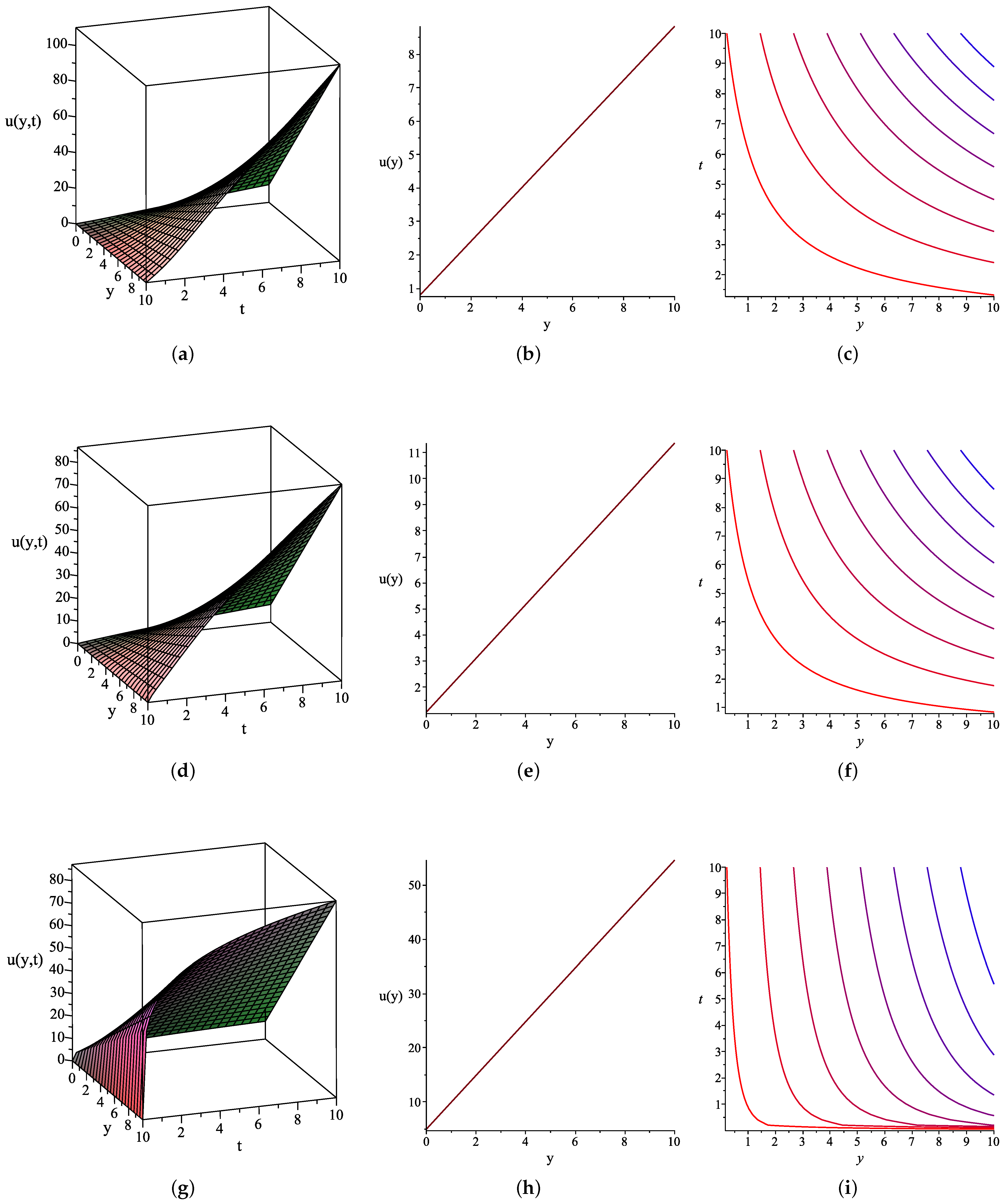
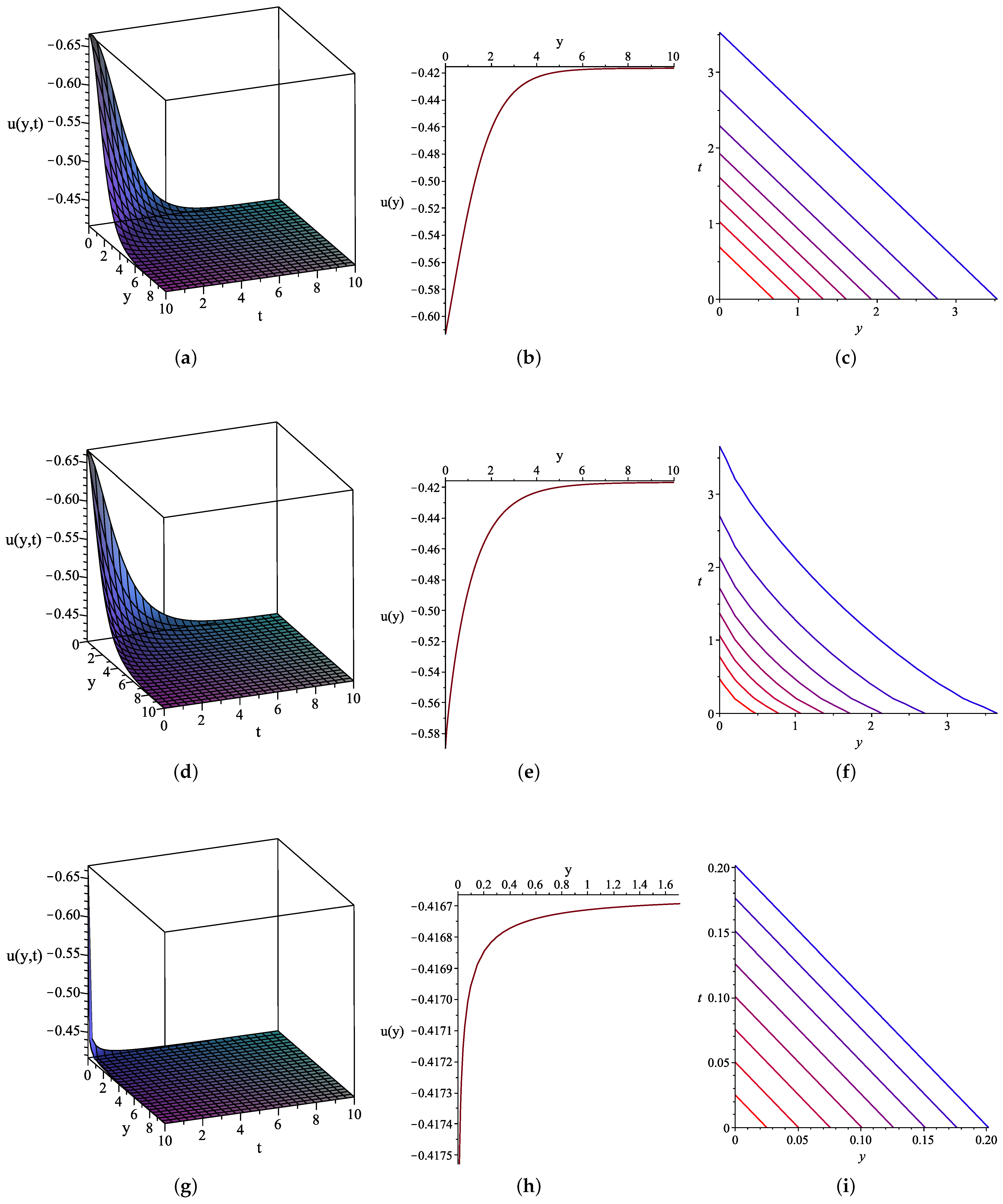
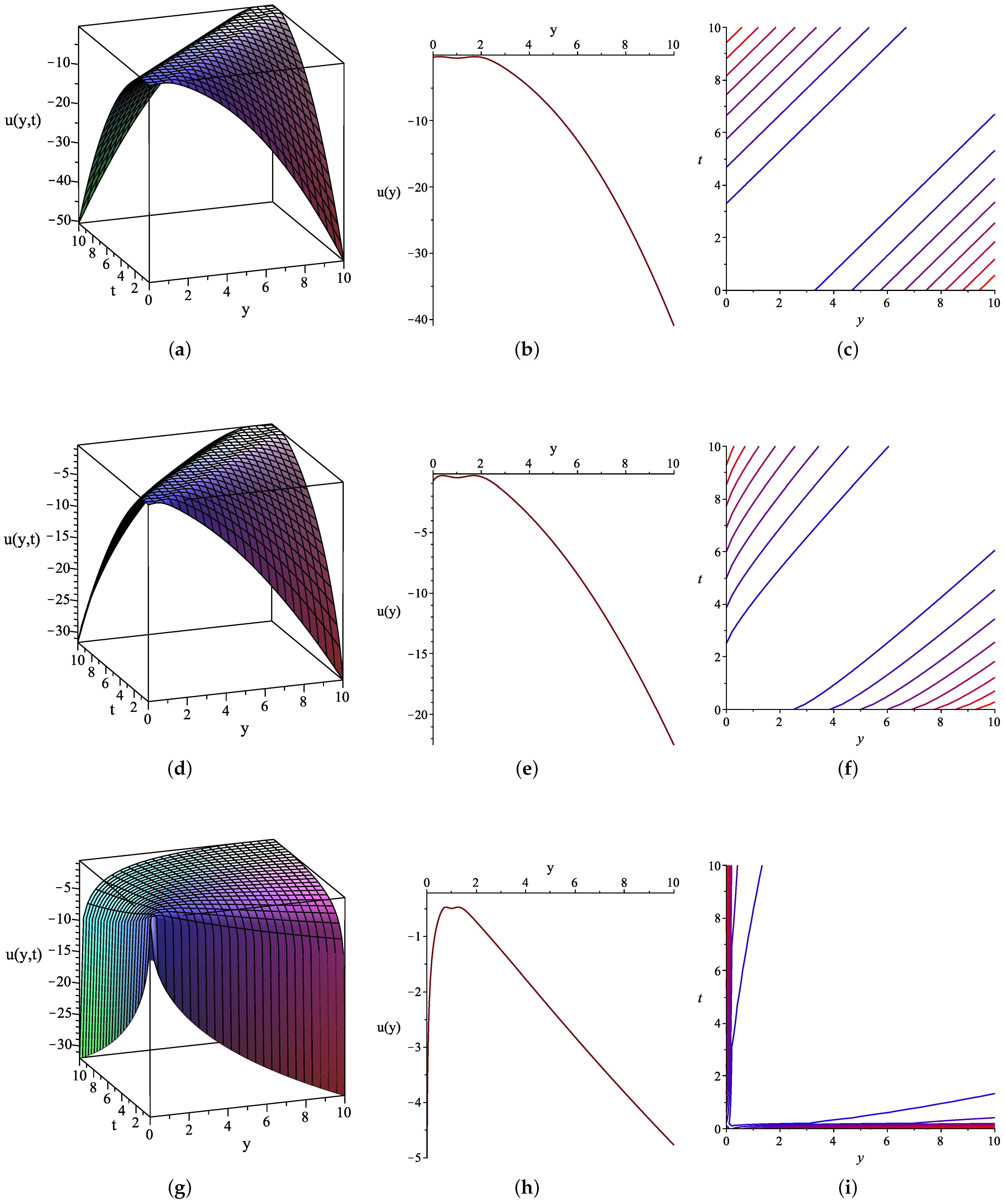
4.2. Conformable Space–Time (2 + 1)-Dimensional Boussinesq Equation

Consider the conformable space–time (2 + 1)-dimensional Boussinesq equation expressed as

$$\frac{{\partial }^{2\alpha }u}{\partial t^{2\alpha }}-\frac{{\partial }^{2\alpha }u}{\partial x^{2\alpha }}-\frac{{\partial }^{2\alpha }u}{\partial y^{2\alpha }}-\frac{{\partial }^{2\alpha }{u}^2}{\partial x^{2\alpha }}-\frac{{\partial }^{4\alpha }u}{\partial x^{4\alpha }}=0,0<\alpha \le 1.$$

(49)

All of the partial derivatives appearing in Equation (49) are the conformable partial derivatives, for instance, $\frac{{\partial }^{2\alpha }u}{\partial x^{2\alpha }}$ represents the conformable partial derivative of the unknown function $u=u\left(x,y,t\right)$ with respect to the independent variable x of order $2\alpha$. Applying the fractional complex transformations for the variables $t,x,y$ and u as

$$T=c\left(\frac{t^{\alpha }}{\alpha }\right),X=k_1\left(\frac{x^{\alpha }}{\alpha }\right),Y=k_2\left(\frac{y^{\alpha }}{\alpha }\right),u\left(x,y,t\right)=\tilde{u}\left(X,Y,T\right),$$

(50)

where $c,k_1,k_2$ are arbitrary constants and utilizing some properties of the conformable derivative described in Section 2, we have $\frac{{\partial }^{\alpha }u}{\partial t^{\alpha }}=c{\tilde{u}}_T,$$\frac{{\partial }^{\alpha }u}{\partial x^{\alpha }}=k_1{\tilde{u}}_X,$$\frac{{\partial }^{\alpha }u}{\partial y^{\alpha }}=k_2{\tilde{u}}_Y$ and $\frac{{\partial }^{2\alpha }u}{\partial t^{2\alpha }}=\frac{{\partial }^{\alpha }}{\partial t^{\alpha }}\left(\frac{{\partial }^{\alpha }u}{\partial t^{\alpha }}\right)=\frac{{\partial }^{\alpha }}{\partial t^{\alpha }}\left(c{\tilde{u}}_T\right)=c^2{\tilde{u}}_{TT}$. Proceeding in the manner above, the rest terms in (49) can be transformed into integer order partial derivatives and we consequently get the following PDE

$$c^2{\tilde{u}}_{TT}-k_1^2{\tilde{u}}_{XX}-k_2^2{\tilde{u}}_{YY}-2k_1^2{\left({\tilde{u}}_X\right)}^2-2k_1^2\tilde{u}{\tilde{u}}_{XX}-k_1^4{\tilde{u}}_{XXXX}=0.$$

(51)

By the auxiliary equation method, the exact solution form for Equation (51) can be written as

$$\tilde{u}\left(X,Y,T\right)=\sum _{i=0}^m{a}_i\left(Y,T\right){\left(\frac{{\psi }^{\prime }\left(\xi \right)}{\psi \left(\xi \right)}\right)}^i,$$

(52)

where $\xi =\xi \left(X,Y,T\right)$ and $a_i\left(Y,T\right),i=0,1,\dots ,m$ are some functions that are determined at a later step. Alternatively, we can set each coefficient $a_i$ as any function of the old and new variables but we here let $a_i$ be a function of only the new variables Y and T. Similarly, the function $\psi \left(\xi \right)$ is the solution of the Riccati Equation (20). The expressions for $\psi \left(\xi \right)$ and $\frac{{\psi }^{\prime }\left(\xi \right)}{\psi \left(\xi \right)}$ can be found in Equations (21) and (22) (or (23)), respectively.

Denoting $\mathrm{Deg}\left[\tilde{u}\right]=m$ and then utilizing Equation (10) of [33] to balance the degree of the highest order derivative ${\tilde{u}}_{XXXX}$ and of the nonlinear term $\tilde{u}{\tilde{u}}_{XX}$ in (51), we get $\mathrm{Deg}\left[{\tilde{u}}_{XXXX}\right]=m+4=\mathrm{Deg}\left[\tilde{u}{\tilde{u}}_{XX}\right]=m+\left(m+2\right)$ and then $m=2$. Hence, the solution form for Equation (51) can be determined as

$$\tilde{u}\left(X,Y,T\right)=a_2\left(Y,T\right){\left(\frac{{\psi }^{\prime }\left(\xi \right)}{\psi \left(\xi \right)}\right)}^2+a_1\left(Y,T\right)\left(\frac{{\psi }^{\prime }\left(\xi \right)}{\psi \left(\xi \right)}\right)+a_0\left(Y,T\right).$$

(53)

Inserting Equation (53) into Equation (51) along with Equation (20), collecting all of the terms with the same power of $\psi \left(\xi \right)$ together and then equating each of the obtained coefficients to zero, we have a set of partial differential equations in variables $a_0\left(Y,T\right),a_1\left(Y,T\right),a_2\left(Y,T\right),\xi \left(X,Y,T\right)$. Due to the minimalism, only some parts of the resulting PDEs are demonstrated if they are too long. The system of the obtained PDEs can be expressed as follows.

$$\begin{array}{c}\hfill \begin{array}{cc}\hfill {\psi }^0& :c^2{\lambda }^2\frac{{\partial }^2}{\partial T^2}{a}_2\left(Y,T\right)-c^2\lambda \frac{{\partial }^2}{\partial T^2}{a}_1\left(Y,T\right)-k_2^2{\lambda }^2\frac{{\partial }^2}{\partial Y^2}{a}_2\left(Y,T\right)+k_2^2\lambda \frac{{\partial }^2}{\partial Y^2}{a}_1\left(Y,T\right)\hfill \\ & +\dots =0,\hfill \\ \hfill {\psi }^1& :-k_1^2{\lambda }^2{a}_1\left(Y,T\right){\left(\frac{\partial }{\partial X}\xi \left(X,Y,T\right)\right)}^2-4k_2^2{\lambda }^2\frac{\partial }{\partial Y}{a}_2\left(Y,T\right)\frac{\partial }{\partial Y}\xi \left(X,Y,T\right)+\dots =0,\hfill \\ \hfill {\psi }^2& :-4c^2\lambda a_2\left(Y,T\right)\frac{{\partial }^2}{\partial T^2}\xi \left(X,Y,T\right)+4k_1^2\lambda a_2\left(Y,T\right)\frac{{\partial }^2}{\partial X^2}\xi \left(X,Y,T\right)+\dots =0,\hfill \\ \hfill {\psi }^3& :4c^2\frac{\partial }{\partial T}{a}_2\left(Y,T\right)\frac{\partial }{\partial T}\xi \left(X,Y,T\right)-4k_2^2\frac{\partial }{\partial Y}{a}_2\left(Y,T\right)\frac{\partial }{\partial Y}\xi \left(X,Y,T\right)\hfill \\ & +\dots =0,\hfill \\ \hfill {\psi }^4& :396k_1^4\lambda a_2\left(Y,T\right)\frac{{\partial }^2}{\partial X^2}\xi \left(X,Y,T\right){\left(\frac{\partial }{\partial X}\xi \left(X,Y,T\right)\right)}^2\hfill \\ & -6k_2^2{a}_2\left(Y,T\right){\left(\frac{\partial }{\partial Y}\xi \left(X,Y,T\right)\right)}^2+\dots =0,\hfill \\ \hfill {\psi }^5& :-24k_1^4{a}_1\left(Y,T\right){\left(\frac{\partial }{\partial X}\xi \left(X,Y,T\right)\right)}^4-4k_1^2{\left(a_2\left(Y,T\right)\right)}^2\frac{{\partial }^2}{\partial X^2}\xi \left(X,Y,T\right)+\dots =0,\hfill \\ \hfill {\psi }^6& :-120k_1^4{a}_2\left(Y,T\right){\left(\frac{\partial }{\partial X}\xi \left(X,Y,T\right)\right)}^4-20k_1^2{\left(a_2\left(Y,T\right)\right)}^2{\left(\frac{\partial }{\partial X}\xi \left(X,Y,T\right)\right)}^2=0.\hfill \end{array}\end{array}$$

(54)

Solving system (54) with the help of Maple 17 and after removing trivial and redundant solutions, we obtain 14 distinct sets of the unknown functions $a_0\left(Y,T\right),a_1\left(Y,T\right),a_2\left(Y,T\right),$

$\xi \left(X,Y,T\right)$. In consequence, we can write the exact solutions with variable coefficient function forms for Equation (49) using (22) (or (23)) and (53) as follows.

Result 1:

$$\begin{array}{c}\hfill \begin{array}{cc}\hfill a_0\left(Y,T\right)& =F_1\left(-cY-k_{2}T\right)+F_2\left(-cY+k_{2}T\right),a_1\left(Y,T\right)=0,a_2\left(Y,T\right)=0,\hfill \\ \hfill \xi \left(X,Y,T\right)& =\xi \left(X,Y,T\right),\hfill \end{array}\end{array}$$

(55)

where $F_1,F_2$ are arbitrary functions of $-cY-k_{2}T$ and $-cY+k_{2}T$, respectively. Thus, the exact solution of Equation (49) is

$$u_1\left(x,y,t\right)=F_1\left(-cY-k_{2}T\right)+F_2\left(-cY+k_{2}T\right),$$

(56)

where $T=c\left(\frac{t^{\alpha }}{\alpha }\right)$ and $Y=k_2\left(\frac{y^{\alpha }}{\alpha }\right)$.

Result 2:

$$\begin{array}{c}\hfill \begin{array}{cc}\hfill a_0\left(Y,T\right)=& F_1\left(-cY-k_{2}T\right)+F_2\left(-cY+k_{2}T\right),a_1\left(Y,T\right)=F_3\left(-cY-k_{2}T\right)\hfill \\ & +F_4\left(-cY+k_{2}T\right),a_2\left(Y,T\right)=0,\xi \left(X,Y,T\right)=C_1,\hfill \end{array}\end{array}$$

(57)

where $C_1$ is an arbitrary constant and $F_1,F_3$ are arbitrary functions of $-cY-k_{2}T$ and $F_2,F_4$ are arbitrary functions of $-cY+k_{2}T$. Thus, the exact solution for Equation (49) is shown as

$$\begin{array}{cc}\hfill u_2\left(x,y,t\right)=& -F_1\left(-cY-k_{2}T\right)\frac{d{\lambda }^2{e}^{\lambda \xi }}{1+d\lambda e^{\lambda \xi }}+F_2\left(-cY+k_{2}T\right)\frac{d{\lambda }^2{e}^{\lambda \xi }}{1+d\lambda e^{\lambda \xi }}\hfill \\ \hfill & +F_3\left(-cY-k_{2}T\right)+F_4\left(-cY+k_{2}T\right),\hfill \end{array}$$

(58)

where $\xi =\xi \left(X,Y,T\right)=C_1,T=c\left(\frac{t^{\alpha }}{\alpha }\right)$ and $Y=k_2\left(\frac{y^{\alpha }}{\alpha }\right)$. If we select $d=\frac{1}{\lambda }$, then $u_2\left(x,y,t\right)$ in (58) becomes

$$\begin{array}{cc}\hfill u_2\left(x,y,t\right)=& -\frac{\lambda }{2}\left(F_1\left(-cY-k_{2}T\right)+F_2\left(-cY+k_{2}T\right)\right)\left(1+\tanh \left(\frac{1}{2}\lambda C_1\right)\right)\hfill \\ \hfill & +F_3\left(-cY-k_{2}T\right)+F_4\left(-cY+k_{2}T\right).\hfill \end{array}$$

(59)

Result 3:

$$\begin{array}{c}\hfill \begin{array}{cc}\hfill a_0\left(Y,T\right)& =F_1\left(-cY-k_{2}T\right)+F_2\left(-cY+k_{2}T\right),a_1\left(Y,T\right)=F_3\left(\frac{cY+k_{2}T}{k_2}\right),\hfill \\ \hfill a_2\left(Y,T\right)& =0,\xi \left(X,Y,T\right)=F_3\left(\frac{cY+k_{2}T}{k_2}\right),\hfill \end{array}\end{array}$$

(60)

where $F_1,F_2,F_3$ are arbitrary functions of $-cY-k_{2}T,-cY+k_{2}T$ and $\frac{cY+k_{2}T}{k_2}$, respectively. Thus, the exact solution of Equation (49) is as follows

$$u_3\left(x,y,t\right)=-\frac{d{\lambda }^2{e}^{\lambda \xi }}{1+d\lambda e^{\lambda \xi }}{F}_3\left(\frac{cY+k_{2}T}{k_2}\right)+F_1\left(-cY-k_{2}T\right)+F_2\left(-cY+k_{2}T\right),$$

(61)

where $\xi =\xi \left(X,Y,T\right)=F_3\left(\frac{cY+k_{2}T}{k_2}\right),T=c\left(\frac{t^{\alpha }}{\alpha }\right)$ and $Y=k_2\left(\frac{y^{\alpha }}{\alpha }\right)$. When $d=\frac{1}{\lambda }$, then $u_3\left(x,y,t\right)$ in (61) turns out to be

$$\begin{array}{cc}\hfill u_3\left(x,y,t\right)=& -\frac{\lambda }{2}\left(1+\tanh \left(\frac{1}{2}\lambda F_3\left(\frac{cY+k_{2}T}{k_2}\right)\right)\right)F_3\left(\frac{cY+k_{2}T}{k_2}\right)\hfill \\ \hfill & +F_1\left(-cY-k_{2}T\right)+F_2\left(-cY+k_{2}T\right).\hfill \end{array}$$

(62)

Result 4:

$$\begin{array}{c}\hfill a_0\left(Y,T\right)=\frac{1}{12}{\lambda }^2{C}_2-\frac{1}{2},a_1\left(Y,T\right)=\lambda C_2,a_2\left(Y,T\right)=C_2,\xi \left(X,Y,T\right)=C_1,\end{array}$$

(63)

where $C_1,C_2$ are arbitrary constants. So, the exact solution of Equation (49) is

$$u_4\left(x,y,t\right)=C_2{\left(\frac{d{\lambda }^2{e}^{\lambda \xi }}{1+d\lambda e^{\lambda \xi }}\right)}^2-\lambda C_2{\left(\frac{d{\lambda }^2{e}^{\lambda \xi }}{1+d\lambda e^{\lambda \xi }}\right)}^2+\frac{1}{12}{\lambda }^2{C}_2-\frac{1}{2},$$

(64)

where $\xi =\xi \left(X,Y,T\right)=C_1$. If $d=\frac{1}{\lambda }$, then $u_4\left(x,y,t\right)$ in (64) is transformed into

$$u_4\left(x,y,t\right)=\frac{1}{4}{\lambda }^2{C}_2{\left(1+\tan \mathrm{h}\left(\frac{1}{2}\lambda C_1\right)\right)}^2-\frac{1}{2}{\lambda }^2{C}_2\left(1+\tan \mathrm{h}\left(\frac{1}{2}\lambda C_1\right)\right)+\frac{1}{12}{\lambda }^2{C}_2-\frac{1}{2}.$$

(65)

Result 5:

$$\begin{array}{c}\hfill \begin{array}{cc}\hfill a_0\left(Y,T\right)& =\frac{1}{2}\frac{c^2{C}_1^2-{\lambda }^2{k}_1^4{C}_2^4-k_1^2{C}_2^2}{k_1^2{C}_2^2},a_1\left(Y,T\right)=-6\lambda k_1^2{C}_2^2,a_2\left(Y,T\right)=-6k_1^2{C}_2^2,\hfill \\ \hfill \xi \left(X,Y,T\right)& =C_{2}X+C_{1}T+C_3,\hfill \end{array}\end{array}$$

(66)

where $C_1,C_2,C_3$ are arbitrary constants. Thus, the exact solution of Equation (49) is expressed as

$$u_5\left(x,y,t\right)=-6k_1^2{C}_2^2{\left(\frac{d{\lambda }^2{e}^{\lambda \xi }}{1+d\lambda e^{\lambda \xi }}\right)}^2+6\lambda k_1^2{C}_2^2\left(\frac{d{\lambda }^2{e}^{\lambda \xi }}{1+d\lambda e^{\lambda \xi }}\right)+\frac{1}{2}\frac{c^2{C}_1^2-{\lambda }^2{k}_1^4{C}_2^4-k_1^2{C}_2^2}{k_1^2{C}_2^2},$$

(67)

where $\xi =\xi \left(X,Y,T\right)=C_{2}X+C_{1}T+C_3,T=c\left(\frac{t^{\alpha }}{\alpha }\right)$ and $X=k_1\left(\frac{x^{\alpha }}{\alpha }\right)$. If we choose $d=\frac{1}{\lambda }$, then $u_5\left(x,y,t\right)$ in (67) becomes

$$\begin{array}{cc}\hfill u_5\left(x,y,t\right)=& -\frac{3}{2}{\lambda }^2{k}_1^2{C}_2^2{\left(1+\tanh \left(\frac{1}{2}\lambda \left(C_{2}X+C_{1}T+C_3\right)\right)\right)}^2\hfill \\ \hfill & +3{\lambda }^2{k}_1^2{C}_2^2\left(1+\tanh \left(\frac{1}{2}\lambda \left(C_{2}X+C_{1}T+C_3\right)\right)\right)\hfill \\ \hfill & +\frac{1}{2}\frac{c^2{C}_1^2-{\lambda }^2{k}_1^4{C}_2^4-k_1^2{C}_2^2}{k_1^2{C}_2^2}.\hfill \end{array}$$

(68)

Result 6:

$$a_0\left(Y,T\right)=\frac{1}{12}{\lambda }^2{C}_1-\frac{1}{2},a_1\left(Y,T\right)=\lambda C_1,a_2\left(Y,T\right)=C_1,\xi \left(X,Y,T\right)=F_1\left(\frac{cY+k_{2}T}{k_2}\right),$$

(69)

where $C_1$ is an arbitrary constant and $F_1$ is an arbitrary function of $\frac{cY+k_{2}T}{k_2}$. Hence, the exact solution of Equation (49) for this case is

$$u_6\left(x,y,t\right)=C_1{\left(\frac{d{\lambda }^2{e}^{\lambda \xi }}{1+d\lambda e^{\lambda \xi }}\right)}^2-\lambda C_1\left(\frac{d{\lambda }^2{e}^{\lambda \xi }}{1+d\lambda e^{\lambda \xi }}\right)+\frac{1}{12}{\lambda }^2{C}_1-\frac{1}{2},$$

(70)

where $\xi =\xi \left(X,Y,T\right)=F_1\left(\frac{cY+k_{2}T}{k_2}\right),T=c\left(\frac{t^{\alpha }}{\alpha }\right)$ and $Y=k_2\left(\frac{y^{\alpha }}{\alpha }\right)$. If $d=\frac{1}{\lambda }$, then $u_6\left(x,y,t\right)$ in (70) becomes

$$\begin{array}{cc}\hfill u_6\left(x,y,t\right)=& \frac{1}{4}{\lambda }^2{C}_1{\left(1+\lambda \tanh \left(\frac{1}{2}{F}_1\left(\frac{cY+k_{2}T}{k_2}\right)\right)\right)}^2\hfill \\ \hfill & -\frac{1}{2}{\lambda }^2{C}_1\left(1+\lambda \tanh \left(\frac{1}{2}{F}_1\left(\frac{cY+k_{2}T}{k_2}\right)\right)\right)+\frac{1}{12}{\lambda }^2{C}_1-\frac{1}{2}.\hfill \end{array}$$

(71)

Result 7:

$$\begin{array}{c}\hfill \begin{array}{cc}\hfill a_0\left(Y,T\right)& =\frac{1}{2}{\lambda }^2{k}_1^2{C}_1^2-\frac{1}{2},a_1\left(Y,T\right)=-6\lambda k_1^2{C}_1^2,a_2\left(Y,T\right)=-6k_1^2{C}_1^2\hfill \\ \hfill \xi \left(X,Y,T\right)& =C_{1}X+F_1\left(\frac{cY+k_{2}T}{k_2}\right),\hfill \end{array}\end{array}$$

(72)

where $C_1$ is an arbitrary constant and $F_1$ is an arbitrary function of $\frac{cY+k_{2}T}{k_2}$. Thus, the exact solution of Equation (49) is expressed as

$$u_7\left(x,y,t\right)=-6k_1^2{C}_1^2{\left(\frac{d{\lambda }^2{e}^{\lambda \xi }}{1+d\lambda e^{\lambda \xi }}\right)}^2+6\lambda k_1^2{C}_1^2\left(\frac{d{\lambda }^2{e}^{\lambda \xi }}{1+d\lambda e^{\lambda \xi }}\right)+\frac{1}{2}{\lambda }^2{k}_1^2{C}_1^2-\frac{1}{2},$$

(73)

where $\xi =\xi \left(X,Y,T\right)=C_{1}X+F_1\left(\frac{cY+k_{2}T}{k_2}\right),T=c\left(\frac{t^{\alpha }}{\alpha }\right),X=k_1\left(\frac{x^{\alpha }}{\alpha }\right)$ and $Y=k_2\left(\frac{y^{\alpha }}{\alpha }\right)$.

If $d=\frac{1}{\lambda }$, then $u_7\left(x,y,t\right)$ in (73) becomes

$$\begin{array}{cc}\hfill u_7\left(x,y,t\right)=& -\frac{3}{2}{\lambda }^2{k}_1^2{C}_1^2{\left(1+\tanh \left(\frac{1}{2}\lambda \left(C_{1}X+F_1\left(\frac{cY+k_{2}T}{k_2}\right)\right)\right)\right)}^2\hfill \\ & +3{\lambda }^2{k}_1^2{C}_1^2\left(1+\tanh \left(\frac{1}{2}\lambda \left(C_{1}X+F_1\left(\frac{cY+k_{2}T}{k_2}\right)\right)\right)\right)-\frac{1}{2}{\lambda }^2{k}_1^2{C}_1^2-\frac{1}{2}.\hfill \end{array}$$

(74)

Result 8:

$$\begin{array}{c}\hfill \begin{array}{cc}\hfill a_0\left(Y,T\right)& =\frac{1}{2}\frac{c^2{C}_1^2-{\lambda }^2{k}_1^4{C}_2^4-k_1^2{C}_2^2-k_2^2{C}_3^2}{k_1^2{C}_2^2},a_1\left(Y,T\right)=-6\lambda k_1^2{C}_2^2,\hfill \\ \hfill a_2\left(Y,T\right)& =-6k_1^2{C}_2^2,\xi \left(X,Y,T\right)=C_{2}X+C_{3}Y+C_{1}T+C_4,\hfill \end{array}\end{array}$$

(75)

where $C_1,C_2,C_3,C_4$ are arbitrary constants. Thus, the exact solution of Equation (49) is read as

$$\begin{array}{c}\hfill \begin{array}{cc}\hfill u_8\left(x,y,t\right)=& -6k_1^2{C}_2^2{\left(\frac{d{\lambda }^2{e}^{\lambda \xi }}{1+d\lambda e^{\lambda \xi }}\right)}^2+6\lambda k_1^2{C}_2^2\left(\frac{d{\lambda }^2{e}^{\lambda \xi }}{1+d\lambda e^{\lambda \xi }}\right)\hfill \\ & +\frac{1}{2}\frac{c^2{C}_1^2-{\lambda }^2{k}_1^4{C}_2^4-k_1^2{C}_2^2-k_2^2{C}_3^2}{k_1^2{C}_1^2},\hfill \end{array}\end{array}$$

(76)

where $\xi =\xi \left(X,Y,T\right)=C_{2}X+C_{3}Y+C_{1}T+C_4,T=c\left(\frac{t^{\alpha }}{\alpha }\right),X=k_1\left(\frac{x^{\alpha }}{\alpha }\right)$ and $Y=k_2\left(\frac{y^{\alpha }}{\alpha }\right)$. If $d=\frac{1}{\lambda }$, then $u_8\left(x,y,t\right)$ in (76) becomes

$$\begin{array}{cc}\hfill u_8\left(x,y,t\right)=& -\frac{3}{2}{\lambda }^2{k}_1^2{C}_2^2{\left(1+\tanh \left(\frac{1}{2}\lambda \left(C_{2}X+C_{3}Y+C_{1}T+C_4\right)\right)\right)}^2\hfill \\ \hfill & +3{\lambda }^2{k}_1^2{C}_2^2\left(1+\tanh \left(\frac{1}{2}\lambda \left(C_{2}X+C_{3}Y+C_{1}T+C_4\right)\right)\right)\hfill \\ \hfill & +\frac{1}{2}\frac{c^2{C}_1^2-{\lambda }^2{k}_1^4{C}_2^4-k_1^2{C}_2^2-k_2^2{C}_3^2}{k_1^2{C}_2^2}.\hfill \end{array}$$

(77)

Result 9:

$$\begin{array}{c}\hfill \begin{array}{cc}\hfill a_0\left(Y,T\right)& =\frac{1}{2}\frac{-{\lambda }^2{k}_1^4{C}_1^4-k_1^2{C}_1^2-4c^2{k}_2^2{C}_2{F}_1^{\prime }\left(-cY+k_{2}T\right)}{k_1^2{C}_1^2},a_1\left(Y,T\right)=-6\lambda k_1^2{C}_1^2,\hfill \\ \hfill a_2\left(Y,T\right)& =-6k_1^2{C}_1^2,\xi \left(X,Y,T\right)=C_{1}X++c{C}_{2}Y+k_2{C}_{2}T+C_3+F_1\left(-cY+k_{2}T\right),\hfill \end{array}\end{array}$$

(78)

where $C_1,C_2,C_3$ are arbitrary constants and $F_1$ is an arbitrary function of $-cY+k_{2}T$. Therefore, the exact solution of Equation (49) is

$$\begin{array}{cc}\hfill u_9\left(x,y,t\right)=& -6k_1^2{C}_1^2{\left(\frac{d{\lambda }^2{e}^{\lambda \xi }}{1+d\lambda e^{\lambda \xi }}\right)}^2+6\lambda k_1^2{C}_1^2\left(\frac{d{\lambda }^2{e}^{\lambda \xi }}{1+d\lambda e^{\lambda \xi }}\right)\hfill \\ \hfill & +\frac{1}{2}\frac{-{\lambda }^2{k}_1^4{C}_1^4-k_1^2{C}_1^2-4c^2{k}_2^2{C}_2{F}_1^{\prime }\left(-cY+k_{2}T\right)}{k_1^2{C}_1^2},\hfill \end{array}$$

(79)

where $\xi =\xi \left(X,Y,T\right)=C_{1}X++c{C}_{2}Y+k_2{C}_{2}T+C_3+F_1\left(-cY+k_{2}T\right),T=c\left(\frac{t^{\alpha }}{\alpha }\right),X=k_1\left(\frac{x^{\alpha }}{\alpha }\right)$ and $Y=k_2\left(\frac{y^{\alpha }}{\alpha }\right)$. When $d=\frac{1}{\lambda }$, the solution $u_9\left(x,y,t\right)$ in (79) is transformed as

$$\begin{array}{cc}\hfill u_9\left(x,y,t\right)=& -\frac{3}{2}{\lambda }^2{k}_1^2{C}_1^2{\left(1+\tanh \left(\frac{1}{2}\lambda \left(C_{1}X++c{C}_{2}Y+k_2{C}_{2}T+C_3+F_1\left(-cY+k_{2}T\right)\right)\right)\right)}^2\hfill \\ & +3{\lambda }^2{k}_1^2{C}_1^2\left(1+\tanh \left(\frac{1}{2}\lambda \left(C_{1}X++c{C}_{2}Y+k_2{C}_{2}T+C_3+F_1\left(-cY+k_{2}T\right)\right)\right)\right)\hfill \\ & +\frac{1}{2}\frac{-{\lambda }^2{k}_1^4{C}_1^4-k_1^2{C}_1^2-4c^2{k}_2^2{C}_2{F}_1^{\prime }\left(-cY+k_{2}T\right)}{k_1^2{C}_1^2}.\hfill \end{array}$$

(80)

Result 10:

$$\begin{array}{c}\hfill \begin{array}{cc}\hfill a_0\left(Y,T\right)& =F_1\left(-cY-k_{2}T\right)+F_2\left(-cY+k_{2}T\right),a_1\left(Y,T\right)=\lambda C_1,a_2\left(Y,T\right)=C_1,\hfill \\ \hfill \xi \left(X,Y,T\right)& =F_3\left(\frac{cY+k_{2}T}{k_2}\right),\hfill \end{array}\end{array}$$

(81)

where $C_1$ is an arbitrary constant and $F_1,F_2,F_3$ are arbitrary functions of $-cY-k_{2}T,$

$-cY+k_{2}T$ and $\frac{cY+k_{2}T}{k_2}$, respectively. Therefore, the exact solution of Equation (49) is

$$u_{10}\left(x,y,t\right)=C_1{\left(\frac{d{\lambda }^2{e}^{\lambda \xi }}{1+d\lambda e^{\lambda \xi }}\right)}^2-\lambda C_1\left(\frac{d{\lambda }^2{e}^{\lambda \xi }}{1+d\lambda e^{\lambda \xi }}\right)+F_1\left(-cY-k_{2}T\right)+F_2\left(-cY+k_{2}T\right),$$

(82)

where $\xi =\xi \left(X,Y,T\right)=F_3\left(\frac{cY+k_{2}T}{k_2}\right),T=c\left(\frac{t^{\alpha }}{\alpha }\right)$ and $Y=k_2\left(\frac{y^{\alpha }}{\alpha }\right)$. If $d=\frac{1}{\lambda }$, then the solution $u_{10}\left(x,y,t\right)$ in (82) becomes

$$\begin{array}{cc}\hfill u_{10}\left(x,y,t\right)=& \frac{1}{4}{\lambda }^2{C}_1{\left(1+\tanh \left(\frac{1}{2}\lambda F_3\left(\frac{cY+k_{2}T}{k_2}\right)\right)\right)}^2\hfill \\ \hfill & -\frac{1}{2}{\lambda }^2{C}_1\left(1+\tanh \left(\frac{1}{2}\lambda F_3\left(\frac{cY+k_{2}T}{k_2}\right)\right)\right)+F_1\left(-cY-k_{2}T\right)\hfill \\ \hfill & +F_2\left(-cY+k_{2}T\right).\hfill \end{array}$$

(83)

Result 11:

$$\begin{array}{c}\hfill \begin{array}{cc}\hfill a_0\left(Y,T\right)& =F_1\left(-cY-k_{2}T\right)+F_2\left(-cY+k_{2}T\right),a_1\left(Y,T\right)=\lambda F_3\left(\frac{cY+k_{2}T}{k_2}\right),\hfill \\ \hfill a_2\left(Y,T\right)& =F_3\left(\frac{cY+k_{2}T}{k_2}\right),\xi \left(X,Y,T\right)=F_3\left(\frac{cY+k_{2}T}{k_2}\right),\hfill \end{array}\end{array}$$

(84)

where $F_1,F_2,F_3$ are arbitrary functions of $-cY-k_{2}T,-cY+k_{2}T$ and $\frac{cY+k_{2}T}{k_2}$, respectively. Thus, the exact solution of Equation (49) is expressed as

$$\begin{array}{cc}\hfill u_{11}\left(x,y,t\right)=& {\left(\frac{d{\lambda }^2{e}^{\lambda \xi }}{1+d\lambda e^{\lambda \xi }}\right)}^2{F}_3\left(\frac{cY+k_{2}T}{k_2}\right)-\lambda \frac{d{\lambda }^2{e}^{\lambda \xi }}{1+d\lambda e^{\lambda \xi }}{F}_5\left(\frac{cY+k_{2}T}{k_2}\right)\hfill \\ \hfill & +F_1\left(-cY-k_{2}T\right)+F_2\left(-cY+k_{2}T\right),\hfill \end{array}$$

(85)

where $\xi =\xi \left(X,Y,T\right)=F_3\left(\frac{cY+k_{2}T}{k_2}\right),T=c\left(\frac{t^{\alpha }}{\alpha }\right)$ and $Y=k_2\left(\frac{y^{\alpha }}{\alpha }\right)$. If we select $d=\frac{1}{\lambda }$, then the solution $u_{11}\left(x,y,t\right)$ in (85) turns out to be

$$\begin{array}{cc}\hfill u_{11}\left(x,y,t\right)=& \frac{1}{4}{\lambda }^2{F}_3\left(\frac{cY+k_{2}T}{k_2}\right){\left(1+\tanh \left(\frac{1}{2}\lambda F_3\left(\frac{cY+k_{2}T}{k_2}\right)\right)\right)}^2\hfill \\ \hfill & -\frac{1}{2}{\lambda }^2{F}_3\left(\frac{cY+k_{2}T}{k_2}\right)\left(1+\tanh \left(\frac{1}{2}\lambda F_3\left(\frac{cY+k_{2}T}{k_2}\right)\right)\right)\hfill \\ \hfill & +F_1\left(-cY-k_{2}T\right)+F_2\left(-cY+k_{2}T\right).\hfill \end{array}$$

(86)

Result 12:

$$\begin{array}{c}\hfill \begin{array}{cc}\hfill a_0\left(Y,T\right)& =-\frac{1}{2}{\lambda }^2{k}_1^2{\left(F_1\left(\frac{cY+k_{2}T}{k_2}\right)\right)}^2,a_1\left(Y,T\right)=-6\lambda k_1^2{\left(F_1\left(\frac{cY+k_{2}T}{k_2}\right)\right)}^2,\hfill \\ \hfill a_2\left(Y,T\right)& =-6k_1^2{\left(F_1\left(\frac{cY+k_{2}T}{k_2}\right)\right)}^2,\hfill \\ \hfill \xi \left(X,Y,T\right)& =F_1\left(\frac{cY+k_{2}T}{k_2}\right)X+F_2\left(\frac{cY+k_{2}T}{k_2}\right),\hfill \end{array}\end{array}$$

(87)

where $F_1,F_2$ are arbitrary functions of $\frac{cY+k_{2}T}{k_2}$. Thus, the exact solution for Equation (49) is as follows

$$\begin{array}{cc}\hfill u_{12}\left(x,y,t\right)=& -6k_1^2{\left(\frac{d{\lambda }^2{e}^{\lambda \xi }}{1+d\lambda e^{\lambda \xi }}\right)}^2{\left(F_1\left(\frac{cY+k_{2}T}{k_2}\right)\right)}^2\hfill \\ \hfill & -6\lambda k_1^2\left(\frac{d{\lambda }^2{e}^{\lambda \xi }}{1+d\lambda e^{\lambda \xi }}\right){\left(F_1\left(\frac{cY+k_{2}T}{k_2}\right)\right)}^2\hfill \\ \hfill & +\frac{1}{2}{\lambda }^2{k}_1^2{\left(F_1\left(\frac{cY+k_{2}T}{k_2}\right)\right)}^2-\frac{1}{2},\hfill \end{array}$$

(88)

where $\xi =\xi \left(X,Y,T\right)=F_1\left(\frac{cY+k_{2}T}{k_2}\right)X+F_2\left(\frac{cY+k_{2}T}{k_2}\right),T=c\left(\frac{t^{\alpha }}{\alpha }\right),X=k_1\left(\frac{x^{\alpha }}{\alpha }\right),Y=k_2\left(\frac{y^{\alpha }}{\alpha }\right)$. If $d=\frac{1}{\lambda }$, then $u_{12}\left(x,y,t\right)$ in (88) is transformed into

$$\begin{array}{cc}\hfill u_{12}\left(x,y,t\right)=& -\frac{3}{2}{\lambda }^2{k}_1^2{\left(F_1\left(\frac{cY+k_{2}T}{k_2}\right)\right)}^2\left(1+\tanh \left(\frac{1}{2}\lambda \left(F_1\left(\frac{cY+k_{2}T}{k_2}\right)X\right.\right.\right.\hfill \\ \hfill & {\left.\left.\left.+F_2\left(\frac{cY+k_{2}T}{k_2}\right)\right)\right)\right)}^2\hfill \\ \hfill & +3{\lambda }^2{k}_1^2{\left(F_1\left(\frac{cY+k_{2}T}{k_2}\right)\right)}^2\left(1+\tanh \left(\frac{1}{2}\lambda \left(F_1\left(\frac{cY+k_{2}T}{k_2}\right)X\right.\right.\right.\hfill \\ \hfill & \left.\left.\left.+F_2\left(\frac{cY+k_{2}T}{k_2}\right)\right)\right)\right)-\frac{1}{2}{\lambda }^2{k}_1^2{\left(F_1\left(\frac{cY+k_{2}T}{k_2}\right)\right)}^2-\frac{1}{2}.\hfill \end{array}$$

(89)

Result 13:

$$\begin{array}{c}\hfill \begin{array}{cc}& a_0\left(Y,T\right)=F_1\left(-cY-k_{2}T\right)+F_2\left(-cY+k_{2}T\right),a_1\left(Y,T\right)=\lambda \left(F_3\left(-cY-k_{2}T\right)\right.\hfill \\ & \left.+F_4\left(-cY+k_{2}T\right)\right),a_2\left(Y,T\right)=\frac{a_1\left(Y,T\right)}{\lambda },\xi \left(X,Y,T\right)=C_1,\hfill \end{array}\end{array}$$

(90)

where $C_1$ is an arbitrary constant and $F_1,F_3$ are arbitrary functions of $-cY-k_{2}T$ and $F_2,F_4$ are arbitrary functions of $-cY+k_{2}T$. Thus, the exact solution of Equation (49) is

$$\begin{array}{cc}\hfill u_{13}\left(x,y,t\right)=& \left(F_3\left(-cY-k_{2}T\right)+F_4\left(-cY+k_{2}T\right)\right){\left(\frac{d{\lambda }^2{e}^{\lambda \xi }}{1+d\lambda e^{\lambda \xi }}\right)}^2\hfill \\ \hfill & -\lambda \left(F_3\left(-cY-k_{2}T\right)+F_4\left(-cY+k_{2}T\right)\right)\left(\frac{d{\lambda }^2{e}^{\lambda \xi }}{1+d\lambda e^{\lambda \xi }}\right)\hfill \\ \hfill & +F_1\left(-cY-k_{2}T\right)+F_2\left(-cY+k_{2}T\right),\hfill \end{array}$$

(91)

where $\xi =\xi \left(X,Y,T\right)=C_1,T=c\left(\frac{t^{\alpha }}{\alpha }\right)$ and $Y=k_2\left(\frac{y^{\alpha }}{\alpha }\right)$. If $d=\frac{1}{\lambda }$, then $u_{13}\left(x,y,t\right)$ in (91) becomes

$$\begin{array}{cc}\hfill u_{13}\left(x,y,t\right)=& \frac{1}{4}{\lambda }^2\left(F_3\left(-cY-k_{2}T\right)+F_4\left(-cY+k_{2}T\right)\right){\left(1+\tanh \left(\frac{1}{2}\lambda C_1\right)\right)}^2\hfill \\ \hfill & -\frac{1}{2}{\lambda }^2\left(F_3\left(-cY-k_{2}T\right)+F_4\left(-cY+k_{2}T\right)\right)\left(1+\tanh \left(\frac{1}{2}\lambda C_1\right)\right)\hfill \\ \hfill & +F_1\left(-cY-k_{2}T\right)+F_2\left(-cY+k_{2}T\right).\hfill \end{array}$$

(92)

Result 14:

$$\begin{array}{c}\hfill \begin{array}{cc}\hfill a_0\left(Y,T\right)& =F_1\left(-cY-k_{2}T\right)+F_2\left(-cY+k_{2}T\right),a_1\left(Y,T\right)=F_3\left(\frac{cY+k_{2}T}{k_2}\right),\hfill \\ \hfill a_2\left(Y,T\right)& =F_3\left(\frac{cY+k_{2}T}{k_2}\right),\xi \left(X,Y,T\right)=F_3\left(\frac{cY+k_{2}T}{k_2}\right),\hfill \end{array}\end{array}$$

(93)

where $F_1,F_2,F_3$ are arbitrary functions of $-cY-k_{2}T,-cY+k_{2}T$ and $\frac{cY+k_{2}T}{k_2}$, respectively. Thus, the exact solution of Equation (49) is

$$\begin{array}{cc}\hfill u_{14}\left(x,y,t\right)=& {\left(\frac{d{\lambda }^2{e}^{\lambda \xi }}{1+d\lambda e^{\lambda \xi }}\right)}^2{\left(F_3\left(\frac{cY+k_{2}T}{k_2}\right)\right)}^2-\left(\frac{d{\lambda }^2{e}^{\lambda \xi }}{1+d\lambda e^{\lambda \xi }}\right){\left(F_3\left(\frac{cY+k_{2}T}{k_2}\right)\right)}^2\hfill \\ \hfill & +F_1\left(-cY-k_{2}T\right)+F_2\left(-cY+k_{2}T\right),\hfill \end{array}$$

(94)

where $\xi =\xi \left(X,Y,T\right)=F_3\left(\frac{cY+k_{2}T}{k_2}\right),T=c\left(\frac{t^{\alpha }}{\alpha }\right)$ and $Y=k_2\left(\frac{y^{\alpha }}{\alpha }\right)$. When we choose $d=\frac{1}{\lambda }$, then the solution $u_{14}\left(x,y,t\right)$ in (94) turns out to be

$$\begin{array}{cc}\hfill u_{14}\left(x,y,t\right)=& \frac{1}{4}{\lambda }^2{F}_3\left(\frac{cY+k_{2}T}{k_2}\right){\left(1+\tanh \left(\frac{1}{2}\lambda F_3\left(\frac{cY+k_{2}T}{k_2}\right)\right)\right)}^2\hfill \\ \hfill & -\frac{1}{2}\lambda F_3\left(\frac{cY+k_{2}T}{k_2}\right)\left(1+\tanh \left(\frac{1}{2}\lambda F_3\left(\frac{cY+k_{2}T}{k_2}\right)\right)\right)\hfill \\ \hfill & +F_1\left(-cY-k_{2}T\right)+F_2\left(-cY+k_{2}T\right).\hfill \end{array}$$

(95)

Some selected exact solutions, which are obtained using the auxiliary equation method, of the conformable space–time (2 + 1)-dimensional Boussinesq equation expressed in (49) is graphically presented by considering some effect of distinct values of the fractional order $\alpha$. Their graphical representations include the 3-D, 2-D and contour plots on a particular domain. In Figure 4, the graphs of $u_6\left(x,y,t\right)$ in (71) are portrayed by setting $c=\lambda =k_2=C_1=1$ and $F_1\left(z\right)=z$. Specifically, Figure 4a–c shows the 3-D plot on $0\le y,t\le 10$, the 2-D plot with $0\le y\le 10,t=1$ and the contour plot of $u_6\left(x,y,t\right)$ when $\alpha =1$. In the same manner, the 3-D, 2-D and contour graphs of $u_6\left(x,y,t\right)$ when $\alpha =0.8$ and $\alpha =0.2$ are displayed in Figure 4d–f and g–i, respectively.

Furthermore, Figure 5 shows the associated plots for $u_8\left(x,y,t\right)$ in (77) evaluated when $c=\lambda =k_1=k_2=C_1=C_2=C_3=C_4=1$. In particular, Figure 5a–c shows the 3-D graph on $0\le y,t\le 10,x=1$, the 2-D graph with $0\le y\le 10,x=t=1$ and the contour graph of $u_8\left(x,y,t\right)$ when $\alpha =1$. In the same manner, Figure 5d–f and g–i are portrayed using $\alpha =0.8$ and $\alpha =0.2,$ respectively. The exact solution $u_9\left(x,y,t\right)$ in (80) with $c=\lambda =k_1=k_2=C_1=C_2=C_3=1$ and $F_1\left(z\right)=z$ is drawn as the 3-D, 2-D and contour graphs in Figure 6. Specifically, $\alpha =1$ is employed for plotting the 3-D graph on $0\le y,t\le 10,x=1$, the 2-D graph with $0\le y\le 10,x=t=1$ and the contour graph of $u_9\left(x,y,t\right)$ as demonstrated in Figure 6a–c. Proceeding in a similar manner, Figure 6d–f and g–i are portrayed when $\alpha =0.8$ and $\alpha =0.2,$ respectively. Lastly, the 3-D, 2-D and contour plots of the solution $u_{12}\left(x,y,t\right)$ in (89) are exhibited in Figure 7 using $c=\lambda =k_1=k_2=1$ and $F_1\left(z\right)=F_2\left(z\right)=z$. In particular, Figure 7a–c shows the 3-D plot on $0\le y,t\le 10,x=1$, the 2-D graph with $0\le y\le 10,x=t=1$ and the contour plot of $u_{12}\left(x,y,t\right)$ when $\alpha =1$. Proceeding in like manner, the 3-D, 2-D and contour graphs of $u_{12}\left(x,y,t\right)$ when $\alpha =0.8$ and $\alpha =0.2$ are shown in Figure 7d–f and g–i, respectively.

5. Conclusions and Outlook

The brief algorithm of an auxiliary equation method for solving a nonlinear conformable PDE for an exact solution, in which its coefficients are in the form of variable functions, comprises the following steps. Firstly, the conformable PDE is converted into an integer order PDE via some fractional complex transformations. Secondly, we assume that an exact solution of the transformed equation is in the form of a polynomial, which has variable function coefficients and is associated with a solution of an auxiliary equation such that the Riccati equation. The degree of such a polynomial solution can be determined using the homogeneous balance principle. Thirdly, we use symbolic software packages such as Maple 17 to solve a system of PDEs expressed in terms of the variable function coefficients. Such a system of the PDEs is derived by inserting the known solution form into the integer order PDE and then equating all coefficients of the solution of the auxiliary equation to be zero. Finally, the exact solution of the original equation can be formulated via the known variable function coefficients. According to the use of the method, we have obtained eight different exact solutions for the conformable time (2 + 1)-dimensional Kadomtsev–Petviashvili Equation (16) and fourteen exact solutions for the conformable space–time (2 + 1)-dimensional Boussinesq Equation (49). In particular, most of the obtained exact solutions for both equations can be written in terms of hyperbolic tangent functions if we set $d=\frac{1}{\lambda }$. As a result, some graphical representations of the obtained outcomes demonstrate certain physical behaviors, for example, the graphs of $u_2\left(x,y,t\right)$ in (30) are characterized as an inclined bell-shaped solitary wave solution and the plots of $u_8\left(x,y,t\right)$ in (77) represent a 1-soliton solitary wave solution. Since our exact solutions for the two equations have the variable coefficients including constant coefficients, then the obtained results are new and reported here for the first time. Of course, all of the exact solutions for both equations constructed using the method have been checked by substituting them back into their corresponding equations with the help of Maple 17.

In summary, an auxiliary equation method along with the use of symbolic computation packages is a reliable, efficient and convenient tool for extracting exact solutions with variable coefficient function forms for the interesting NPDEs arising in applied sciences and engineering. Such solution forms include the case of constant coefficients which has been already used for assuming an exact solution form for other existing methods. Changing function forms for variable coefficients in the assumed exact solution such as replacing $a_i(y,T)$ with $a_i(x,y,T)$ or a use of other auxiliary equations different from the Riccati equation could consequently produce more and various exact solutions for the NPDEs.

References

1. Ali, M.R.; Ma, W.X. New exact solutions of nonlinear (3+1)-dimensional Boiti-Leon-Manna-Pempinelli equation. Adv. Math. Phys. 2019, 2019, 9801638. [Google Scholar] [CrossRef] [Green Version]
2. Gepreel, K.A. Analytical Methods for Nonlinear Evolution Equations in Mathematical Physics. Mathematics 2020, 8, 2211. [Google Scholar] [CrossRef]
3. Alharbi, A.; Almatrafi, M.B. Exact and numerical solitary wave structures to the variant Boussinesq system. Symmetry 2020, 12, 1473. [Google Scholar] [CrossRef]
4. Li, Y.; Teng, Z.; Hu, C.; Ge, Q. Global stability of an epidemic model with age-dependent vaccination, latent and relapse. Chaos Solitons Fractals 2017, 105, 195–207. [Google Scholar] [CrossRef]
5. Pananu, K.; Sungnul, S.; Sirisubtawee, S.; Phongthanapanich, S. Convergence and Applications of the Implicit Finite Difference Method for Advection-Diffusion-Reaction Equations. IAENG Int. J. Comput. Sci. 2020, 47, 645–663. [Google Scholar]
6. Miah, M.M.; Ali, H.S.; Akbar, M.A.; Seadawy, A.R. New applications of the two variable (G′/G,1/G)–expansion method for closed form traveling wave solutions of integro-differential equations. J. Ocean. Eng. Sci. 2019, 4, 132–143. [Google Scholar] [CrossRef]
7. Yokus, A.; Durur, H.; Ahmad, H.; Thounthong, P.; Zhang, Y.F. Construction of exact traveling wave solutions of the Bogoyavlenskii equation by (G′/G,1/G)–expansion and (1/G′)–expansion techniques. Results Phys. 2020, 19, 103409. [Google Scholar] [CrossRef]
8. Yokuş, A.; Durur, H.; Abro, K.A.; Kaya, D. Role of Gilson–Pickering equation for the different types of soliton solutions: A nonlinear analysis. Eur. Phys. J. Plus 2020, 135, 1–19. [Google Scholar] [CrossRef]
9. Wan, P.; Manafian, J.; Ismael, H.F.; Mohammed, S.A. Investigating one-, two-, and triple-wave solutions via multiple exp-function method arising in engineering sciences. Adv. Math. Phys. 2020, 2020. [Google Scholar] [CrossRef]
10. Hosseini, K.; Mirzazadeh, M.; Osman, M.; Al Qurashi, M.; Baleanu, D. Solitons and Jacobi elliptic function solutions to the complex Ginzburg–Landau equation. Front. Phys. 2020, 8, 225. [Google Scholar] [CrossRef]
11. Tala-Tebue, E.; Rezazadeh, H.; Eslami, M.; Bekir, A. New approach to model coupled nerve fibers and exact solutions of the system. Chin. J. Phys. 2019, 62, 179–186. [Google Scholar] [CrossRef]
12. Yue, C.; Lu, D.; Arshad, M.; Nasreen, N.; Qian, X. Bright-Dark and Multi Solitons Solutions of (3+1)-Dimensional Cubic-Quintic Complex Ginzburg–Landau Dynamical Equation with Applications and Stability. Entropy 2020, 22, 202. [Google Scholar] [CrossRef] [Green Version]
13. Pinar, Z. The combination of conservation laws and auxiliary equation method. Int. J. Appl. Comput. Math. 2020, 6, 1–7. [Google Scholar] [CrossRef]
14. Mahak, N.; Akram, G. The modified auxiliary equation method to investigate solutions of the perturbed nonlinear Schrödinger equation with Kerr law nonlinearity. Optik 2020, 207, 164467. [Google Scholar] [CrossRef]
15. Rezazadeh, H.; Korkmaz, A.; Eslami, M.; Mirhosseini-Alizamini, S.M. A large family of optical solutions to Kundu–Eckhaus model by a new auxiliary equation method. Opt. Quantum Electron. 2019, 51, 1–12. [Google Scholar] [CrossRef]
16. Akbulut, A.; Kaplan, M. Auxiliary equation method for time-fractional differential equations with conformable derivative. Comput. Math. Appl. 2018, 75, 876–882. [Google Scholar] [CrossRef]
17. Khater, M.M.; Seadawy, A.R.; Lu, D. New optical soliton solutions for nonlinear complex fractional Schrödinger equation via new auxiliary equation method and novel (G/G,1/G)-expansion method. Pramana 2018, 90, 1–20. [Google Scholar] [CrossRef]
18. Meng, F.; Feng, Q. Exact solutions with variable coefficient function forms for conformable fractional partial differential equations by an auxiliary equation method. Adv. Math. Phys. 2018, 2018. [Google Scholar] [CrossRef] [Green Version]
19. Lu, D.; Seadawy, A.R.; Iqbal, M. Mathematical methods via construction of traveling and solitary wave solutions of three coupled system of nonlinear partial differential equations and their applications. Results Phys. 2018, 11, 1161–1171. [Google Scholar] [CrossRef]
20. Pinar, Z.; Kocak, H. Exact solutions for the third-order dispersive-Fisher equations. Nonlinear Dyn. 2018, 91, 421–426. [Google Scholar] [CrossRef]
21. Owyed, S.; Abdou, M.; Abdel-Aty, A.H.; Ray, S.S. New optical soliton solutions of nolinear evolution equation describing nonlinear dispersion. Commun. Theor. Phys. 2019, 71, 1063. [Google Scholar] [CrossRef]
22. Durur, H.; Tasbozan, O.; Kurt, A. New analytical solutions of conformable time fractional bad and good modified Boussinesq equations. Appl. Math. Nonlinear Sci. 2020, 5, 447–454. [Google Scholar] [CrossRef]
23. Xu, Z.; Chen, H.; Dai, Z. Rogue wave for the (2 + 1)-dimensional Kadomtsev–Petviashvili equation. Appl. Math. Lett. 2014, 37, 34–38. [Google Scholar] [CrossRef]
24. Ghanbari, B.; Liu, J.G. Exact solitary wave solutions to the (2 + 1)-dimensional generalised Camassa–Holm–Kadomtsev–Petviashvili equation. Pramana 2020, 94, 1–11. [Google Scholar] [CrossRef]
25. Zhang, Z.; Yang, X.; Li, W.; Li, B. Trajectory equation of a lump before and after collision with line, lump, and breather waves for (2 + 1)-dimensional Kadomtsev–Petviashvili equation. Chin. Phys. B 2019, 28, 110201. [Google Scholar] [CrossRef]
26. Lu, D.; Seadawy, A.R.; Ahmed, I. Applications of mixed lump-solitons solutions and multi-peaks solitons for newly extended (2 + 1)-dimensional Boussinesq wave equation. Mod. Phys. Lett. 2019, 33, 1950363. [Google Scholar] [CrossRef]
27. Feng, L.L.; Tian, S.F.; Zhang, T.T. Bäcklund transformations, nonlocal symmetries and soliton–cnoidal interaction solutions of the (2 + 1)-dimensional Boussinesq Equation. Bull. Malays. Math. Sci. Soc. 2020, 43, 141–155. [Google Scholar] [CrossRef]
28. Khalil, R.; Horani, M.A.; Yousef, A.; Sababheh, M. A new definition of fractional derivative. J. Comput. Appl. Math. 2014, 264, 65–70. [Google Scholar] [CrossRef]
29. Kumar, D.; Seadawy, A.R.; Joardar, A.K. Modified Kudryashov method via new exact solutions for some conformable fractional differential equations arising in mathematical biology. Chin. J. Phys. 2018, 56, 75–85. [Google Scholar] [CrossRef]
30. Rezazadeh, H.; Korkmaz, A.; Eslami, M.; Vahidi, J.; Asghari, R. Traveling wave solution of conformable fractional generalized reaction Duffing model by generalized projective Riccati equation method. Opt. Quantum Electron. 2018, 50, 1–13. [Google Scholar] [CrossRef]
31. Sirisubtawee, S.; Koonprasert, S.; Sungnul, S. Some Applications of the (G/G,1/G)–Expansion Method for Finding Exact Traveling Wave Solutions of Nonlinear Fractional Evolution Equations. Symmetry 2019, 11, 952. [Google Scholar] [CrossRef] [Green Version]
32. Sirisubtawee, S.; Koonprasert, S.; Sungnul, S.; Leekparn, T. Exact traveling wave solutions of the space–time fractional complex Ginzburg–Landau equation and the space-time fractional Phi-4 equation using reliable methods. Adv. Differ. Equ. 2019, 2019, 1–23. [Google Scholar] [CrossRef]
33. Sirisubtawee, S.; Koonprasert, S.; Sungnul, S. New Exact Solutions of the Conformable Space-Time Sharma–Tasso–Olver Equation Using Two Reliable Methods. Symmetry 2020, 12, 644. [Google Scholar] [CrossRef] [Green Version]
34. Topsakal, M.; TaŞcan, F. Exact Travelling Wave Solutions for Space-Time Fractional Klein-Gordon Equation and (2 + 1)-Dimensional Time-Fractional Zoomeron Equation via Auxiliary Equation Method. Appl. Math. Nonlinear Sci. 2020, 5, 437–446. [Google Scholar] [CrossRef]
35. Clarkson, P.A. New similarity solutions for the modified Boussinesq equation. J. Phys. Math. Gen. 1989, 22, 2355. [Google Scholar] [CrossRef]
36. Clarkson, P.A.; Kruskal, M.D. New similarity reductions of the Boussinesq equation. J. Math. Phys. 1989, 30, 2201–2213. [Google Scholar] [CrossRef]
Figure 1. Associated plots of u 2 ( x , y , t ) in Equation (30) obtained using the auxiliary equation method: (ac) 3-D plot, 2-D plot and contour plot, respectively when α = 1 ; (df) 3-D plot, 2-D plot and contour plot, respectively when α = 0.8 ; (gi) 3-D plot, 2-D plot and contour plot, respectively when α = 0.2 .
Computation 09 00031 g001
Figure 2. Associated plots of u 6 ( x , y , t ) in Equation (42) obtained using the auxiliary equation method: (ac) 3-D plot, 2-D plot and contour plot, respectively when α = 1 ; (df) 3-D plot, 2-D plot and contour plot, respectively when α = 0.8 ; (gi) 3-D plot, 2-D plot and contour plot, respectively when α = 0.2 .
Computation 09 00031 g002
Figure 3. Associated plots of u 7 ( x , y , t ) in Equation (45) obtained using the auxiliary equation method: (ac) 3-D plot, 2-D plot and contour plot, respectively when α = 1 ; (df) 3-D plot, 2-D plot and contour plot, respectively when α = 0.8 ; (gi) 3-D plot, 2-D plot and contour plot, respectively when α = 0.2 .
Computation 09 00031 g003
Figure 4. Associated plots of u 6 ( x , y , t ) in Equation (71) obtained using the auxiliary equation method: (ac) 3-D plot, 2-D plot and contour plot, respectively when α = 1 ; (df) 3-D plot, 2-D plot and contour plot, respectively when α = 0.8 ; (gi) 3-D plot, 2-D plot and contour plot, respectively when α = 0.2 .
Computation 09 00031 g004
Figure 5. Associated plots of u 8 ( x , y , t ) in Equation (77) obtained using the auxiliary equation method: (ac) 3-D plot, 2-D plot and contour plot, respectively when α = 1 ; (df) 3-D plot, 2-D plot and contour plot, respectively when α = 0.8 ; (gi) 3-D plot, 2-D plot and contour plot, respectively when α = 0.2 .
Computation 09 00031 g005
Figure 6. Associated plots of u 9 ( x , y , t ) in Equation (80) obtained using the auxiliary equation method: (ac) 3-D plot, 2-D plot and contour plot, respectively when α = 1 ; (df) 3-D plot, 2-D plot and contour plot, respectively when α = 0.8 ; (gi) 3-D plot, 2-D plot and contour plot, respectively when α = 0.2 .
Computation 09 00031 g006
Figure 7. Associated plots of u 12 ( x , y , t ) in Equation (89) obtained using the auxiliary equation method: (ac) 3-D plot, 2-D plot and contour plot, respectively when α = 1 ; (df) 3-D plot, 2-D plot and contour plot, respectively when α = 0.8 ; (gi) 3-D plot, 2-D plot and contour plot, respectively when α = 0.2 .
Computation 09 00031 g007
Publisher’s Note: MDPI stays neutral with regard to jurisdictional claims in published maps and institutional affiliations.