Closing the Wearable Gap—Part VI: Human Gait Recognition Using Deep Learning Methodologies

Abstract

A novel wearable solution using soft robotic sensors (SRS) has been investigated to model foot-ankle kinematics during gait cycles. The capacitance of SRS related to foot-ankle basic movements was quantified during the gait movements of 20 participants on a flat surface as well as a cross-sloped surface. In order to evaluate the power of SRS in modeling foot-ankle kinematics, three-dimensional (3D) motion capture data was also collected for analyzing gait movement. Three different approaches were employed to quantify the relationship between the SRS and the 3D motion capture system, including multivariable linear regression, an artificial neural network (ANN), and a time-series long short-term memory (LSTM) network. Models were compared based on the root mean squared error (RMSE) of the prediction of the joint angle of the foot in the sagittal and frontal plane, collected from the motion capture system. There was not a significant difference between the error rates of the three different models. The ANN resulted in an average RMSE of 3.63, being slightly more successful in comparison to the average RMSE values of 3.94 and 3.98 resulting from multivariable linear regression and LSTM, respectively. The low error rate of the models revealed the high performance of SRS in capturing foot-ankle kinematics during the human gait cycle.

1. Introduction

Gait recognition systems are non-invasive biometric technologies that can be used to analyze the way someone walks. These technologies have applications in both surveillance and healthcare systems. Clinical research has identified clear links between human gait characteristics and different medical conditions and demonstrated their significance not only in clinical disease diagnosis and prevention [1,2,3,4,5,6], but also in the fields of sports [7], rehabilitation [8], training, and robotics [9,10]. The importance of gait analysis in sports is to improve performance as well as to avoid the risk of injuries in athletics [11]. Throughout one gait cycle, each lower extremity passes through two phases: (a) a stance phase and (b) a swing phase. During the stance phase, five different movement stages with corresponding joint angles are executed: (a) initial contact/heel strike (0° of ankle and knee flexion/extension, 20° flexion of the hip joint), (b) foot flat (5° plantar flexion of ankle, 15° of flexion of knee and hip joints), (c) midstance (5° dorsiflexion of ankle, 5° flexion of knee, 0° of hip), (d) heel off (0° of flexion of ankle and knee, 10–20° of hyperextension of hip), and (e) toe-off (20° plantar flexion of ankle, 30° of knee flexion, 10–20° of hyperextension of hip). The second stage—the swing phase—consists of three stages: (a) acceleration (10° plantar flexion of ankle, 30° flexion of knee, 20° of flexion of hip), (b) midswing (0° ankle flexion, 30° flexion of knee and hip), and (c) deceleration (0° of ankle and knee, 30° flexion of hip) [12]. Figure 1 presents the different phases of gait movement.

Optical motion capture analyzes the 3-dimensional (3D) position and motion of a subject using data captured by two or more cameras and has been widely used in different areas. Optical motion capture systems provide an accurate solution for analyzing kinematics and kinetics of the gait cycle and has been considered the gold standard for monitoring gait movement [14,15]; however, they are costly, labor-intensive and their use is restricted to the clinical settings [14,16]. Because this system is only available in clinical settings, implementation of data capture during real-life activities, activities that occur outside the lab, or those that require continuous monitoring are difficult.

Wearable sensors (WS) are another technology that could be joined with the body or wearable objects to monitor the health situation and record human motion activities in real-time [17]. WS could be implemented to assess the human gait cycle, and since they are portable, foot-ankle kinematic analysis can be performed during real-life scenarios. Additionally, WS cost considerably less than a motion capture system. In general, a motion capture system including PC, software, and a model V12 to model V16 Vicon camera system will cost between $125 K and $150 K, while the WS solution used for this study cost roughly $2000. Several types of WS, including accelerometers, gyroscopes, microelectromechanical systems (MEMS), and inertial measurement units (IMUs), have been introduced in the literature.

Accelerometers and gyroscopes could be used together to determine the position and orientation of a moving object by measuring acceleration and angular velocity signals. The history of using accelerometers and gyroscopes in analyzing position and orientation can be tracked back to aerospace studies; however, these technologies could be implemented in analyzing human gait kinematics [18]. Early studies around accelerometers go back to the 1990s when Willemsen et al. [19] and Heyn et al. [20] implemented uniaxial accelerometers for analyzing the movements of the foot, shank, thigh, and pelvis of subjects by Velcro strap attachment; however, their model was only suitable when there were simple motions.

IMUs have been utilized in navigation and attitude estimation of aerial vehicles [21] and they have been implemented for tracking human motion in recent years. IMUs do not suffer from occlusions, but Filippeschi et al. [22] indicated that IMUs have issues with reducing drift, magnetic disturbances, and calibration. Luczak et al. [23] designed a study in order to investigate the use of liquid metal sensors, specifically Liquid Wire sensors, as a potential solution for accurately capturing foot-ankle complex movements such as plantar flexion (PF), dorsiflexion (DF), inversion (INV), and eversion (EVR). The results of this study confirmed the researchers’ hypothesis that soft robotic sensors (SRS) can serve as a substitute for IMU-based solutions attempting to capture specific foot-ankle kinematics.

Several studies have been conducted for evaluating the performance of SRS introduced by Luczak et al. [23] in analyzing human foot-ankle movement [24,25,26]. Saucier et al. [24] investigated the foot-ankle movements in a sitting position and compared SRS against a 3D motion capture system to illustrate the performance of SRS in analyzing joint angles and to determine optimal placement and orientation of the SRS. Chander et al. [25] conducted a study using 10 participants to evaluate the performance of SRS during more complicated movements: slip and trip perturbations. Four different experiments were performed including an unexpected trip, expected trip, unexpected slip, and expected slip. Comparing the SRS result against the 3D motion capture system demonstrated that 71.25% of the trials exhibited a minimal error of less than 4.0 degrees using a linear regression model.

In a more recent study from Saucier et al. [26], a multivariable linear regression model was implemented to investigate four different foot ankle movements including DF, PF, INV, and EVR during the gait cycle in two designed walking surfaces: a flat surface and a cross-sloped surface with 10 degrees incline (in order to increase the intensity of INV and EVR movements). While previous studies used a simple linear model, the data collected from this study revealed that the output of the SRS was coupled to multiple movements. This was determined to be a result of the tri-planar movement of the foot-ankle complex, categorized as supination and pronation, that occurs while a human is walking. Pronation consists of abduction, DF, and EVR, while supination consists of adduction, PF, and INV [27]. When seeing that pronation and supination are natural combinations of ankle movements, Saucier et al. [26] deduced that the output of the SRS mounted to the foot will change based on more than one plane of movement. As a result, more advanced modeling approaches were investigated to handle this behavior.

Wearable technology has attracted much attention in studying human movement and there is a vast amount of literature in this field. Different approaches have been employed to address the problem from statistical analyses, rule-based approaches, and linear regressions to more complicated approaches such as data mining. Additionally, deep learning methods have been developed.

Many supervised and unsupervised algorithms have been utilized by researchers to classify human activities or diagnose a specific condition in human movement. Twelve human activities have been studied by Attal et al. [28] using three inertial sensors. Supervised and unsupervised methods including k-nearest neighbor (k-NN), support vector machines (SVM), Gaussian mixture models (GMM), random forest (RF), k-means, Gaussian mixture models (GMM) and hidden Markov models (HMM) were examined on data acquired from the sensors positioned on the chest, right thigh and left ankle. The fall detection problem has been addressed by many researchers [29,30,31]. Ozdemir et al. [29] addressed the problem of fall detection with six classifiers including k-NN, least squares method, SVM, Bayesian decision making, dynamic time warping, and artificial neural networks (ANNs) with more than 99% accuracy. Shibuya et al. [30] introduced a wireless gait analysis sensor (WGAS) system for real-time fall detection using an SVM. WGAS data has been implemented to analyze data from T4 (fourth thoracic vertebra) and waist movement. The SVM achieved 98.8% and 98.7% fall classification accuracies from data at the T4 and belt positions, respectively. Ojetola et al. [31] identified four different types of falls using two SHIMMER sensor nodes with a C4.5 classifier. They report the precision and recall equal to 81% and 92% respectively. Mazilu et al. [5] considered the application of accelerometer sensors in the detection of freezing of gait (FoG) which is a gait deficit in advanced Parkinson’s disease (PD). Random forest (RF), C4.5, naive Bayes, MLP, AdaBoost with C4.5, and bagging with C4.5 have been employed to model data with the average sensitivity and specificity of more than 95%. Sprager et al. [32] analyzed gait cycles of six participants using accelerometer sensors. The SVM has been implemented to recognize the gait movements of participants with three different speeds and the accuracy of the model was equal to 93%.

In another study conducted by Novak et al. [33], two types of sensors including IMUs and pressure-sensitive insoles were implemented to identify within-subject and subject-independent gait initiation and termination. The classification tree successfully identified gait initiation, especially with subject-independent models. Gait termination also had been detected with 80% accuracy. The results reveal the same performance for both types of sensors in identifying gait initiation, while the IMU was more efficient in gait termination detection.

ANNs and recurrent neural networks (RNN) have been implemented widely on human motion analysis as well as gait analysis, performing a variety of tasks including classification, biomechanical modeling, and prediction of gait parameters [34]. Lafuente et al. [35] provided a feed-forward neural network with one hidden layer for classification of arthrosis patients (including ankle, knee and hip arthrosis) from age-matched control subjects using gait data from force plates. The ANN with an 80% discrimination rate outperformed a Bayes quadratic classifier with a 75% discrimination rate. Sepulveda et al. [36] adapted two separate neural networks with backpropagation to model the relationship between electromyography (EMG) (input) and moments and angles (outputs) for the hip, knee and ankle joints. These two models were successful to provide estimation for joint angle and moment with less than 7% deviation. Gioftsos and Grieve [37] carried out three RNNs for prediction of walking speed and walking conditions. The experiments included data from seven different walking speeds (0.30, 0.45, 0.60, 0.75, 0.90, 1.05, and 1.20 statures s⁻¹) and three different conditions of walking: normal walking, walking with a 3.5 kg mass strapped securely and comfortably to the right ankle, and walking with the right knee fixed in an extended position by means of a knee brace. They also implemented linear discriminant analysis (LDA) to evaluate the performance of RNNs. Results revealed that the performance of RNN models is as good as LDA, and there was not a significant improvement in the results. The authors realized that the sample size was too small for training of RNNs.

For this study, the researchers implement a multivariable linear regression model, a feed-forward neural network and an LSTM network to analyze gait movement. In order to evaluate the accuracy of gait assessment with WS data, the researchers compare this data with the data acquired from the 3D motion capture system. The aim of this study is to predict the 3D motion capture data accurately based on data received from eight SRS and validate SRS against the gold standard, examining the success of SRS in modeling the kinematic foot-ankle data during the gait cycle. The researchers compare the results of the three models to find their strengths and weaknesses during the assessment of SRS-based gait data.

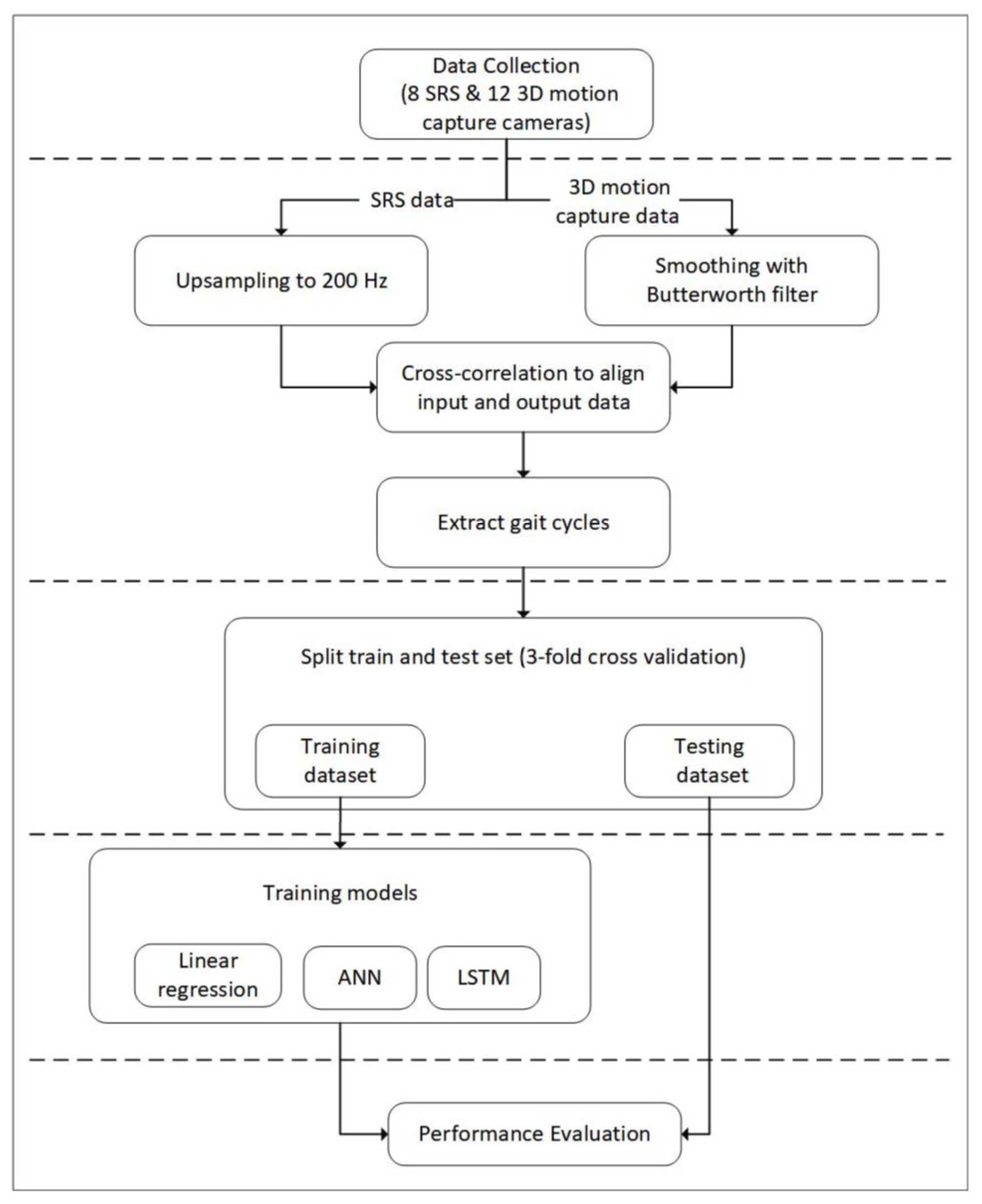
2. Materials and Methods

In the “Closing the Wearable Gap” paper series [24,25,26,38], various scenarios have been designed and tested to further study the capability and efficiency of SRS in tracking lower body movements. In each study, the designed experiments have been modeled and compared to the 3D motion capture system data to investigate the performance of SRS. In Part II [24], four primary foot-ankle complex movements including DF, PF, INV, and EVR have been assessed separately using four sensors placed on the right foot while participants were seated, and best sensor placement has been introduced according to the comparison of SRS data with the 3D motion capture system. Part III [25] designed more dynamic movements, including slip and trip perturbations while there were two different conditions: expected and unexpected. In Part IV [26] of the paper series, which uses the same dataset as the present study, the authors designed two different walking paths including a flat surface and a cross sloped surface with a 10 degrees incline to analyze gait movement. In all these studies, the authors investigate the linear relationship (consisting of a single or multivariable relationship) between the SRS capacitance data and angle orientation in the 3D motion capture system, and the model performance is based only within a specific gait cycle’s dataset. Another study, Part V of the paper series [38], assessed pressure-based SRS against other measurement tools such as pressure mats and force plates but, because this study didn’t specifically assess foot-ankle kinematic data, the methods and data collected were not considered for this present effort. For this study, the researchers create different models including multivariable linear regression, ANN, and LSTM to determine which method explains this relationship most precisely. Further, these models are tested on trials of other datasets to see how well they generalize using cross validation.

2.1. Dataset

A dataset of 20 participants including 10 men and 10 women provided in [26] was collected for this study. In Part IV, participants were chosen so that different shoe sizes be included in the study. The 10 male participants’ heights were in the range of 168–193 cm; their mass was in range of 61–117 kg; and their foot sizes were in the range of 10–13. The 10 female participants’ heights were in the range of 158–168 cm; their mass was in range of 50–113 kg; and their foot sizes were in the range of 5.5–10. Participants had no self-reported history of lower extremity musculoskeletal injuries or surgeries and neuromuscular diseases or disorders have been collected.

In this study, the researchers investigate the data from four SRS (for each foot) placed on the foot-ankle to capture four basic ankle movements—PF, DF, EVR, and INV. Sensors have been mounted on the socks according to the optimal placements introduced in Part II [24]; PF SRS was mounted on the dorsal surface and oriented towards the hallux (big toe) to measure the downward movement of the foot; DF SRS was mounted on the heel of the foot to measure the upward movement of the foot towards the lower leg; INV SRS was mounted directly over the lateral malleolus (bony landmark on the lateral side of the ankle) to measure the movement of the sole (bottom of the foot) towards the midline of the body; EVR SRS was mounted directly over the medial malleolus (bony landmark on the medial side of the ankle).

This data constitutes the input space. Data from the right foot and left foot were analyzed separately; therefore, eight SRS in total were used. Each participant completed two different experiments while wearing a pair of socks with the SRS placed over bony landmarks identified in the results of Part II [24], walking on a flat surface and walking on a cross sloped surface with a 10 degrees slope. Each participant walked six times across each walkway, generating 12 trials in total. During each trial, participants completed two to three complete gait cycles based on their stride length.

The data was categorized based on the foot the data was collected on and what surface was being walked across during the trial. These categories are: walking across the flat surface measuring the left foot (WL); walking across the flat surface measuring the right foot (WR); walking across the surface where there is forced INV, measuring the left foot (IL); walking across the surface where there is forced INV measuring the right foot (IR).

A 3D motion capture system was used to capture gait during the experimental trials. Kinematic data was collected using a 3D motion analysis system that contained 12 Bonita 10 infra-red cameras (Vicon, Oxford, UK), which collected the kinematic data at 200 Hz [26]. Retro-reflective marker clusters were attached bilaterally using nylon straps with Velcro on the dorsal aspect of the foot and shank. MotionMonitor^TM software [39] was used to determine the ankle joint center using the centroid method by placing a measurement sensor on the medial and lateral femoral condyles, the medial and lateral malleoli, and the second distal phalanx [40].

The kinematic variables at the ankle were calculated using MotionMonitor^TM software through the Grood-Suntay angle orientation. The foot and ankle joint centers were defined by putting the tip of the measurement stylus on the medial and lateral malleoli and the distal second phalanx. The shank was used as the reference point in the software to create the foot in the software [41]. Foot and ankle complex movements of PF-DF and INV-EVR were quantified and used as dependent variables.

2.2. Data Preprocessing

A few preprocessing steps have been applied to the dataset to make the data easier to model. Data preprocessing steps in this study follow the same approach taken in reference [26], therefore they will only be briefly mentioned here. The 3D motion capture data was collected at 200 Hz and smoothed with a 30 Hz Butterworth filter. SRS data was initially sampled at 25 Hz, which was then up-sampled to 200 Hz to match the 3D motion capture data. Next, the two datasets were aligned over time using cross-correlation. Finally, individual gait cycles were extracted from each of the trials. Depending on the walking pattern of each participant, two or three complete gait cycles were extracted from each trial.

2.3. Experimental Procedures

In order to model the relationship between SRS and 3D motion capture data, three different approaches have been applied including multivariable linear regression, ANN, and LSTM, which are explained in the following sections. The researchers consider data from each participant separately when developing models. Since the pattern of walking for everyone is unique and there are many factors contributing to the way someone walks, data from different participants should be investigated distinctly [42]. In this paper, eight different models for each participant have been developed to model the relationship among four categories of data (left foot, right foot, flat surface, sloped surface). For each model, four sets of inputs (DF, PF, INV, and EVR SRS) are used to predict two sets of output data (sagittal and frontal plane from motion capture).

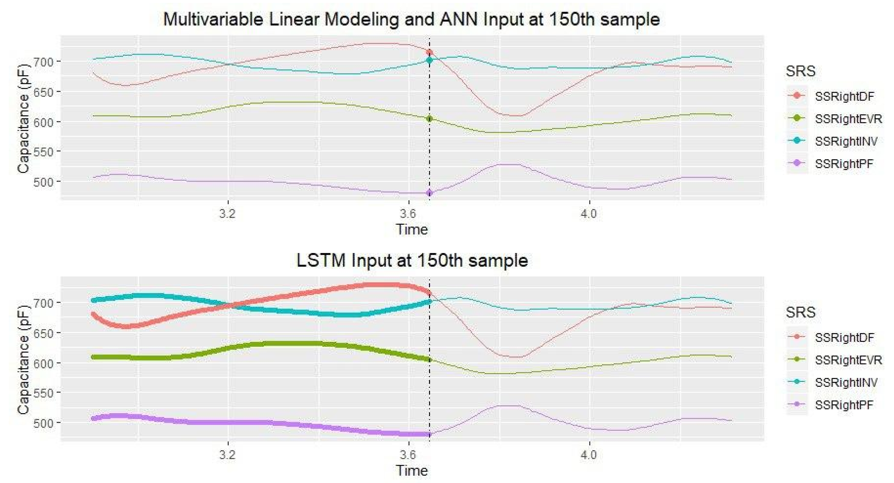
2.3.1. Multivariable Linear Regression

Previous studies using SRS revealed linear modeling could explain the relationship between the SRS data (capacitance) and 3D motion capture data (angle) with a minor error. Multivariable linear regression is like simple linear regression but with multiple independent variables contributing to the dependent variable. In the gait movement, data from all four sensors are used to model each movement since the foot-ankle movements are coupled, so a multivariable linear regression model is needed using Equation (1):

$$Y_i=\alpha +{\beta }_1{x}_i^{\left(1\right)}+{\beta }_2{x}_i^{\left(2\right)}+{\beta }_3{x}_i^{\left(3\right)}+{\beta }_4{x}_i^{\left(4\right)}.$$

(1)

In this equation $Y_i$ is the estimate of the i-th sample from 3D motion capture data, $x_i^{\left(j\right)}$ is the i-th sample from the j-th sensor and ${\beta }_j$ is the coefficient of the j-th sensor. In this regression model, we employed the least-squares approach to fit the best fitting line on the observations in the experiments and predict the α and ${\beta }_j$ coefficients.

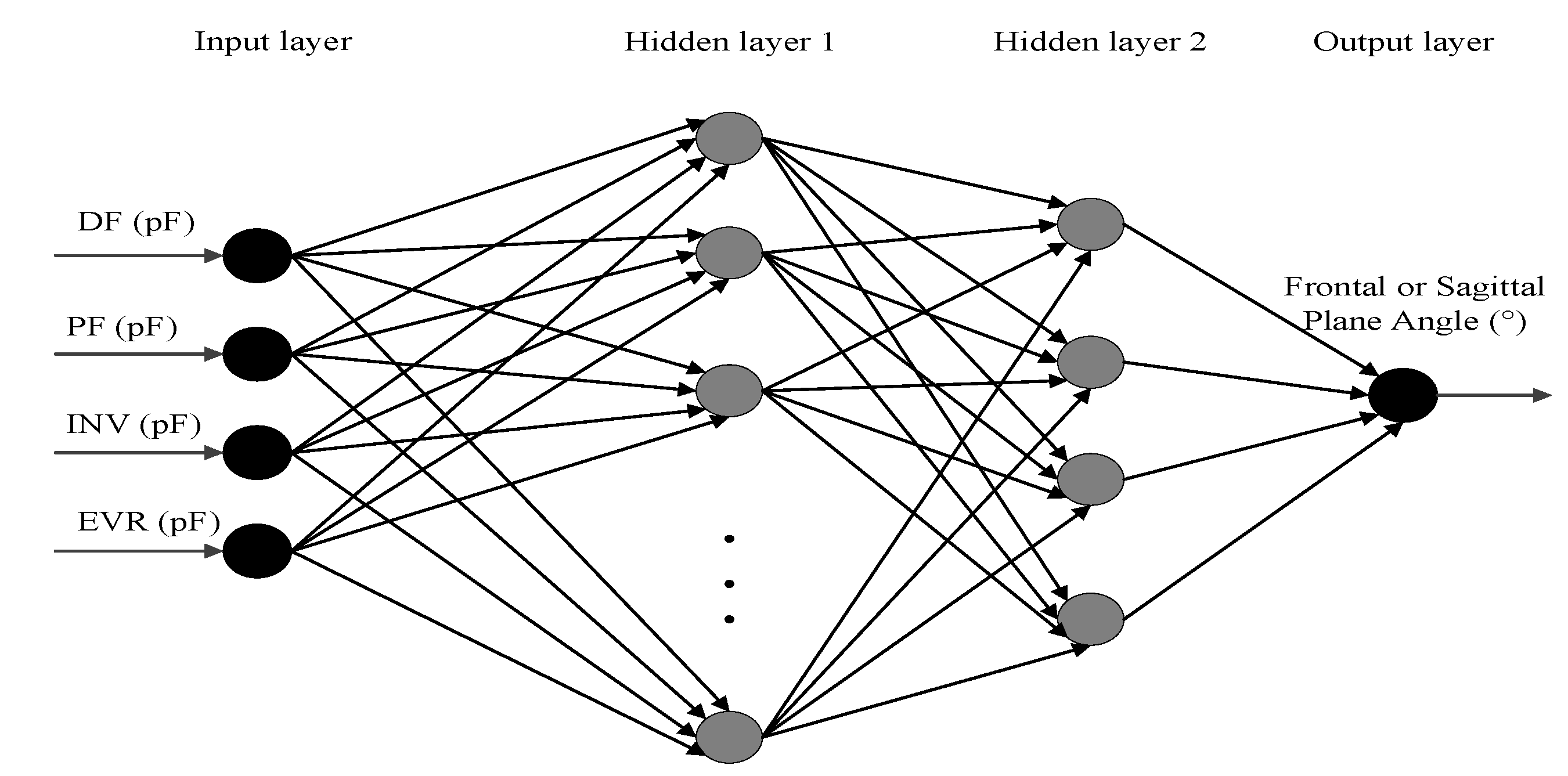
2.3.2. Artificial Neural Network

The ANN or multilayer perceptron (MLP) is a network consisting of several neurons and links between them, which are loosely inspired by the human brain and allows us to model the relationship between dependent and independent variables. ANNs are useful for fitting a model when there are complex hidden patterns on data. An ANN has been carried out for prediction of 3D motion capture data based on the SRS data. This network consists of three segments: the input layer, a hidden layer, and an output layer. In the input layer, there are N neurons equal to the size of the independent attributes in the dataset to enter data into the network. The second part of the ANN consists of a series of hidden layers which are connected according to the weight vectors. They transform the input into something that the output layer can use. Finally, in the output layer, the output of the system will be predicted based on the extracted features from the previous layers.

At the network initialization phase in an untrained model, connections between input and output variables will be established according to the randomly assigned weight vectors. At this stage the model couldn’t perform better than a random prediction model [43]. Through the training process, weight vectors will be updated according to the difference between the prediction of the model and the true target value, and they will be adjusted using the least-squares approach. The number of hidden layers and neurons in each hidden layer depends on the complexity and the degree of nonlinearity in data. If there is no nonlinearity in the data, then there will be no need for hidden layers or nonlinear activations in the neurons. After initializing the network, the network should be trained. In this phase, the input layer processes the input vectors and then passes the outputs through all the layers until they reach the final layer, which predicts the target values. This process is called forward propagation. The performance of the network is then evaluated by the difference between the target value and the prediction of the network for each data point, which will be considered as the loss function. The last phase in the training network is to adjust the network parameters from the model’s errors or misclassifications, which is called backpropagation. In this phase, the error is calculated and distributed through the network to update the weight vectors to converge the network towards better predictions of target values. The error (E) in each epoch (n) of training will be distributed through the network relative to the partial derivative of the error based on each neuron’s weight [44]. The weights will be updated using the Levenberg-Marquardt algorithm and Equation (2):

$$\Delta {\omega }_{ij}\left(n\right)=\eta \frac{\delta E}{\delta {\omega }_{ij}}+\alpha {\omega }_{ij}\left(n-1\right),$$

(2)

where ω_ij indicates the weight of j-th neuron in the i-th layer. The parameters η and α are the learning rate and momentum, respectively. Momentum determines the effect of past weight changes on the direction of weight changes during the training. The network performance improves gradually through repeating forward propagation and backpropagation so that the predictions of the model get as close as possible to the target values.

Different network structures have been tested on the dataset for each participant and input-output combination to determine the best fit for each one. Networks with one and two hidden layers were tested and the number of neurons was between 1 and 10. Figure 2 depicts a general form of an ANN with two hidden layers. We have an input layer with four neurons designed for input attributes including data received from the four SRS placed on the socks. These input variables are fed to the NN for training the weight vectors of the network and the output of the NN is the prediction of the 3D motion capture data. The output layer consists of one neuron producing the output of the network.

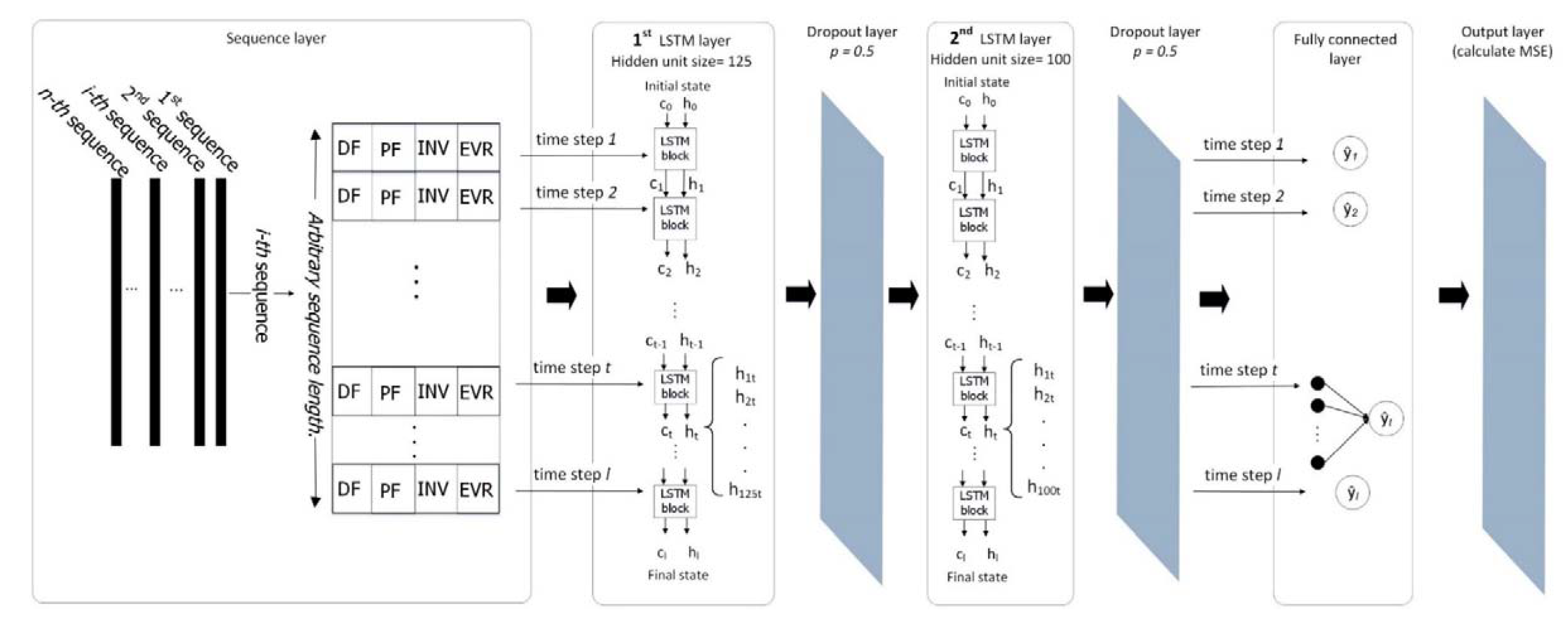
2.3.3. Long Short-Term Memory Network

An LSTM [45] is a special type of RNN architecture that is beneficial when long dependencies exist between samples to tackle the RNNs’ vanishing gradient problem. RNNs have been developed to tackle sequential datasets. In sequential data, there is a meaningful relationship between samples in a dataset, each time step is related to its previous time steps, and RNN cells have a memory that can preserve this relationship. RNNs are more likely to be useful when there are short term dependencies among data, while LSTMs provide networks with a very powerful approach that can handle datasets with long term dependencies. LSTM uses backpropagation through time (BPTT) which is a generalization of backpropagation for training and optimizing weight vectors. Observing the data in this study, the joint angle values of the foot-ankle complex in each time step aren’t separated from each other, and there is a relationship over time between samples. In this section, the network consists of seven layers, and Figure 3 shows the network structure.

Each gait cycle represents a sequence, and the dataset in the form of sequences is the input to the first layer of the network, which is the sequence layer. In the next layer, which uses 125 hidden units, the first LSTM layer is trained. As mentioned before, LSTMs can handle sequences of data.

LSTM has a memory cell (cell state), that enables the LSTM network to remember values over arbitrary time intervals [32], and the network does so using three gates: input gate, forget gate, and output gate. To keep the information from previous time steps, LSTM uses the input vector at time step t and the cell state (contains information from the previous time steps in the current sequence) and hidden state (the output of LSTM block in each time step) of the previous time state (t-1). The output of the LSTM block in each time step at the first LSTM layer would be 125 hidden states.

The dropout layer randomly sets input elements to zero with a given probability and helps prevent the network from overfitting. A dropout layer with p = 0.5 is used as the third layer, which removes half of the inputs received from the previous layer (first LSTM layer). The data is fed into another LSTM layer using 100 hidden units to create a deeper model with more accurate predictions, followed by another dropout layer with p = 0.5. Afterward, a fully connected layer combines all the features (local information) learned by the previous layers and implements the hidden states in each time step to predict the output of models, which is the motion capture output. Finally, the output layer (regression layer) calculates the half-mean-squared-error loss of the predictions. Several different structures have been implemented and among them, this seven-layer network generated the best results. This seven-layer network is implemented to predict the 3D motion capture data based on the gait cycle data gathered by the SRS.

Multivariable linear regression is a simple statistical approach that assumes there is a linear relationship between the input variables and the output variables and fits a linear model over the data. However, if there are nonlinear relationships among the data, ANNs are a more suitable approach to catch the complex structures in the data. Both regression and ANN ignore the relationship between time steps in the dataset and consider only one data point at a time, while LSTMs using the cell memory, preserving the information from previous time steps. Figure 4 depicts the three models’ approaches in using dataset samples during the training phase.

2.4. Validation

In all models explained in previous sections, cross-validation has been used to split the data into a training and testing set in order to train the models and evaluate their performance. In this way, all the trials appear in the test set at least once. There were six trials containing 12–18 sequences (gait cycles) total collected for each experiment. In multivariable linear regression, four trials are randomly selected as training data and the two remaining trials as the test set in each fold to have two-thirds of the data as the training set and one-third as the testing set, which resulted in three-fold cross-validation. The same approach has been conducted for the ANN, except a validation set is needed as well to prevent the model from overtraining. Therefore, four trials are used as the training set, one trial as the validation set, and the remaining trial as the test set. LSTM can handle single data points as well as sequential data, like gait cycles. LSTM is sensitive to the length of the sequence and is not capable of handling the data in the form of long sequences like a complete trial. Therefore, gait cycles are considered as individual sequences of data for training and testing LSTM models. Cross-validation has been implemented to split up the training and testing set for LSTM. In each fold, three gait cycles are randomly selected as the testing dataset and the remaining gait cycles are used as the training dataset, resulting in four-fold, five-fold, and six-fold cross-validation based on the number of completed gaits for each participant. The RMSE was calculated for each model based on the difference between model predictions and actual values acquired by the 3D motion capture system. Figure 5 provides an overview of the performed steps.

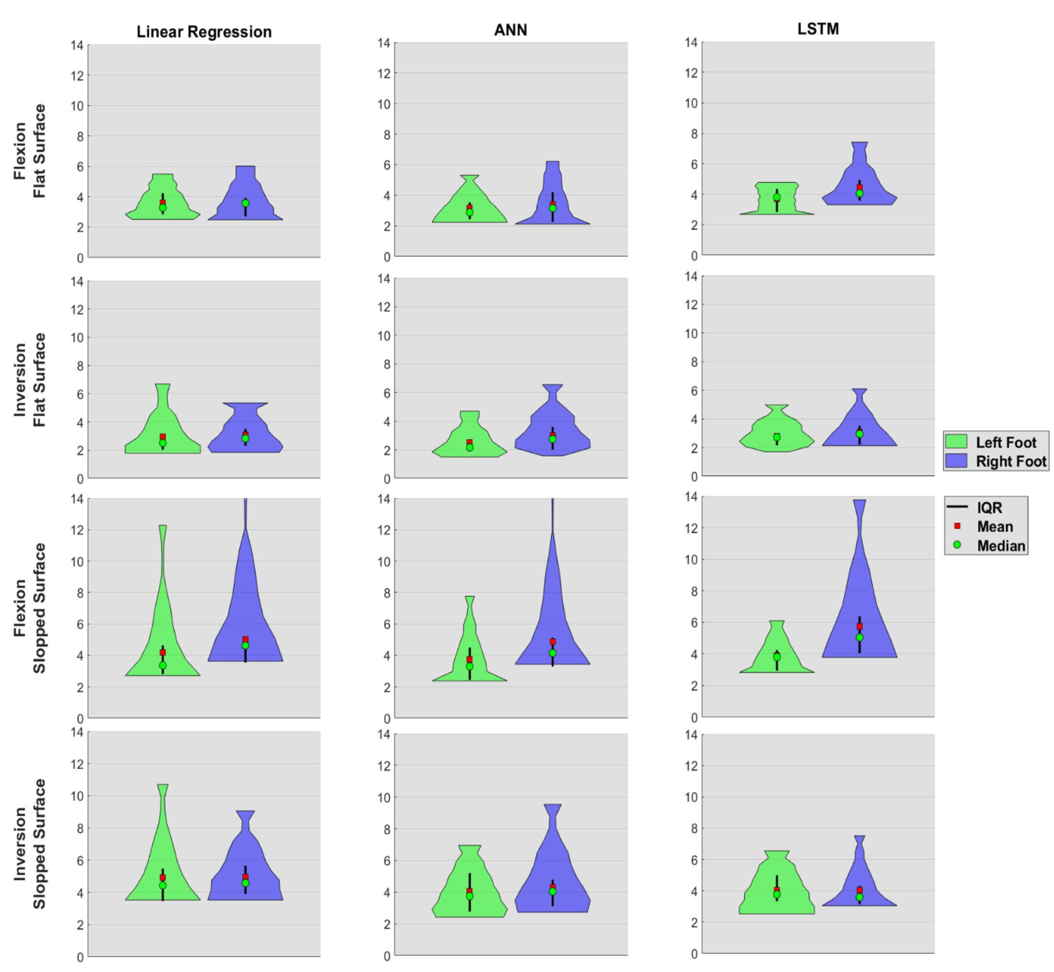
3. Experimental Results and Discussion

The analysis was done with MATLAB^TM R2018a. Models were fit separately for all 20 participants; the mean and standard deviation of RMSE values for all participants are provided in

Table 1. Mean of root mean squared error (RMSE) values in degrees (°) for linear regression, ANN, and LSTM. The lower values indicate better performance (FLX = flexion; INV = inversion).

Model	Data	Flat Surface				Cross Sloped Surface				Overall Mean
		Right foot		Left foot		Right foot		Left foot
		FLX(°)	INV(°)	FLX(°)	INV(°)	FLX(°)	INV(°)	FLX(°)	INV(°)	(°)
Linear regression	Train set	3.27	2.76	3.17	2.51	4.15	4.01	3.27	3.70	3.36
	Test set	3.62	3.09	3.62	2.97	5.02	4.95	4.16	4.93	4.05
ANN	Train set	2.67	2.25	2.53	1.97	3.64	3.17	2.67	2.86	2.72
	Test set	3.40	2.99	3.16	2.51	4.85	4.32	3.74	4.05	3.63
LSTM	Train set	4.58	2.64	3.37	2.46	5.61	3.63	3.78	3.59	3.71
	Test set	4.47	3.08	3.70	2.80	5.74	4.05	4.06	3.89	3.98

and

Table 2. Standard Deviation of RMSE values in degrees (°) for Linear Regression and LSTM. The lower values indicate better performance (FLX = Flexion; INV = Inversion).

Method	Data	Flat Surface				Cross Sloped Surface				Overall Std
		Right foot		Left foot		Right foot		Left foot
		FLX(°)	INV(°)	FLX(°)	INV(°)	FLX(°)	INV(°)	FLX(°)	INV(°)	(°)
Linear regression	Train set	0.85	0.78	0.70	0.95	1.82	1.03	0.89	0.89	0.99
	Test set	1.11	1.03	0.92	1.41	2.92	1.45	2.27	1.87	1.62
ANN	Train set	2.67	2.25	2.53	1.97	3.64	3.17	2.67	2.86	2.72
	Test set	1.28	1.24	0.84	0.97	2.94	1.69	1.49	1.31	1.47
LSTM	Train set	1.11	0.96	0.78	0.66	1.84	1.01	1.09	1.03	1.06
	Test set	1.27	1.01	0.72	0.76	2.38	1.26	1.20	0.96	1.20

respectively. Results for all three approaches including multivariable linear regression, ANN and LSTM are compared in these two tables. According to the results, the ANN provides lower error rates in comparison to the two other methods, and the LSTM performed as the second-best model. However, the LSTM and multivariable linear regression models provide almost the same error, but the LSTM has more uniform RMSE results as it has the lowest standard deviation according to Table 2. The results reveal that there is not a huge difference between errors provided by all three approaches, and all perform well on modeling the relationship between SRS and the 3D motion capture system. Results disclose that it is more challenging for all models to predict the EVR and INV movements which could be explained by the more complex nature of these movements. The angle range for these two movements is more restricted, and there is a high potential for coupling with movements in the sagittal plane, including DF and PF.

A more detailed comparison of the prediction models has been illustrated with the violin plot of the RMSE in Figure 6, which depicts the kernel density distribution of the data at different error values. Prediction errors for each modeling approach are shown in separate columns and the subplots in each row show the results based on the experiment setting (3D motion capture system output; flexion (sagittal plane) and inversion (frontal plane); and designed walking surface; flat surface, and sloped surface). In each subplot, the violin plot of RMSE results from the left foot and right foot are presented with green and blue colors respectively; also, mean (red squares), median (green circles), and interquartile ranges (black line) are illustrated in each plot. The width of each violin plot is related to the percentage of participants having the same error value equal to the value on the y-axis. As we see in the violin plots, the lower part of the plots is wider in most of the subplots, which shows that a greater portion of prediction errors for the 20 participants places within the lower part of the violin plot.

Violin plots of the sloped surface for flexion output on the right foot represent the existence of one or more outliers as these plots have a higher rate of error for all three modeling approaches. In order to identify the potential outliers, we investigated the RMSE errors of 20 participants and realized that participant 4 has a larger RMSE error for this experiment. When reviewing the playback in MotionMonitor^TM, it was noted by the researchers that participant 4 walked flat-footed, which may have been the cause of error. Figure 7 and Figure 8 compare the SRS data for this experiment for participant 4 (as an example of someone who walks flat-footed) and 17 (as an example of someone with normal gait movement) to provide more insight into the potential reasons behind the higher error rate of participant 4 for this particular experiment. Further discussion on potential reasons for outliers can be found in [25]. Excluding data from participant 4 will remedy this situation as seen in Figure 9.

4. Conclusions and Future Work

In this study, the researchers examined three different modeling approaches for prediction of foot-ankle kinematics captured by the 3D motion capture system based on capacitance data collected from SRS during gait movement. The aim of this study is to evaluate the performance of SRS in analyzing gait movement as a substitute for the 3D motion capture system. Results revealed the high performance of the models and the high potential of SRS to be a reliable method for analyzing gait movement. All three models performed well, while the ANN provides prediction errors slightly lower than linear regression and LSTM. LSTM and linear regression provided almost the same RMSE, but the LSTM is computationally expensive. Due to LSTM’s complexity, the researchers were not able to design and apply many structures to find the best fitted structure for each participant. Doing so might improve the LSTM performance.

Another interesting point is that in most of the violin plots we see that the prediction error for the right foot is a little higher than the left foot. This might be related to the mounting of the SRS or 3D motion capture clusters. There were several participants with gait patterns that were challenging for the models to predict; more investigations should be performed to determine if these occurred due to different walking patterns during different trials or if there were some issues regarding how the data was collected.

Future work needs to be done to create generalized models that can predict data for both flat and cross-sloped surfaces simultaneously. In addition to better accuracy with predicting joint angles, deep learning approaches can be investigating using SRS to detect and classify the eight phases of the gait cycle as well as to classify types of gait.

Limitations: In general, deep learning approaches require a large amount of quality data to be successful to train a model that fits the data. In this study we used the dataset from Part IV, and this dataset was not originally collected to be modeled by deep learning algorithms. To collect more data for training deep learning algorithms, performing longer experiments in order to collect more full gait cycles is desired. Furthermore, we strive to develop more generalizable deep learning methods that can generalize and not require per-participant training.

Also, the researchers have only performed data collection on healthy participants to date. In future studies, the researchers plan to use the SRS among participants that do have foot-ankle impairments or injuries, such as chronic ankle instability, with the ultimate goal for the SRS to detect changes in movement kinematics that occur as a result of an injury or long term disability. Deep learning models can become more accurate as larger gait datasets are collected on both healthy participants as well as those with impairments or recovering from injury.

References

1. Hopkins, J.; Son, S.; Kim, H.; Page, G.; Seeley, M. Characterization of Multiple Movement Strategies in Participants with Chronic Ankle Instability. J. Athl. Train. 2019, 54, 698–707. [Google Scholar] [CrossRef] [PubMed] [Green Version]
2. Kim, H.; Son, S.J.; Seeley, M.K.; Hopkins, J.T. Altered movement biomechanics in chronic ankle instability, coper, and control groups: Energy absorption and distribution implications. J. Athl. Train. 2019, 54, 708–717. [Google Scholar] [CrossRef] [PubMed] [Green Version]
3. Son, S.; Kim, H.; Seeley, M.; Hopkins, J. Altered Walking Neuromechanics in Patients with Chronic Ankle Instability. J. Athl. Train. 2019, 54, 684–697. [Google Scholar] [CrossRef] [Green Version]
4. Zeng, W.; Liu, F.; Wang, Q.; Wang, Y.; Ma, L.; Zhang, Y. Parkinson’s disease classification using gait analysis via deterministic learning. Neurosci. Lett. 2016, 633, 268–278. [Google Scholar] [CrossRef]
5. Mazilu, S.; Hardegger, M.; Zhu, Z.; Roggen, D.; Tröster, G.; Plotnik, M.; Hausdorff, J.M. Online detection of freezing of gait with smartphones and machine learning techniques. In Proceedings of the 6th International Conference on Pervasive Computing Technologies for Healthcare and Workshops, San Diego, CA, USA, 21–24 May 2012; pp. 123–130. [Google Scholar]
6. Staranowicz, A.; Brown, G.R.; Mariottini, G.L. Evaluating the accuracy of a mobile Kinect-based gait-monitoring system for fall prediction. In ACM International Conference Proceeding Series; Association for Computing Machinery: New York, NY, USA, 2013 May; pp. 1–4. [Google Scholar]
7. Senanayake, S.M.N.A.; Chong, V.; Chong, J.; Sirisinghe, G.R. Analysis of soccer actions using wireless accelerometers. In Proceedings of the 4th IEEE International Conference on Industrial Informatics, Singapore, 16–18 August 2006; pp. 664–669. [Google Scholar]
8. Ye, M.; Yang, C.; Stanković, V.; Stanković, L.; Kerr, A. A Depth Camera Motion Analysis Framework for Tele-rehabilitation: Motion Capture and Person-Centric Kinematics Analysis. IEEE J. Sel. Top. Signal Process. 2016, 10, 877–887. [Google Scholar] [CrossRef] [Green Version]
9. Hesse, S.; Uhlenbrock, D.; Werner, C.; Bardeleben, A. A mechanized gait trainer for restoring gait in nonambulatory subjects. Arch. Phys. Med. Rehabil. 2000, 81, 1158–1161. [Google Scholar] [CrossRef] [PubMed]
10. Daniel, P.F.P.; Gregory, S.S.M.; Antoinette, R.D.M.P.T. Powered Lower Limb Orthoses for Gait Rehabilitation. Top. Spinal Cord Inj. Rehabil. 2005, 11, 34–49. [Google Scholar]
11. Luczak, T.; Burch, R.; Lewis, E.; Chander, H.; Ball, J. State-of-the-art review of athletic wearable technology: What 113 strength and conditioning coaches and athletic trainers from the USA said about technology in sports. Int. J. Sport. Sci. Coach. 2020, 15, 26–40. [Google Scholar] [CrossRef]
12. Winter, D.; Eng, F.; Isshac, M. A review of kinetic parameters in human walking. In Gait Analysis: Theory and Application; Crak, R.L., Oatis, C.A., Eds.; Mosby-Year Book: Louis MO, USA, 1994; pp. 263–265. [Google Scholar]
13. Cuccurullo, S. Physical Medicine and Rehabilitation Board Review, 1st ed.; Demos Medical Publishing: New York, NY, USA, 2019. [Google Scholar]
14. Fong, D.T.P.; Chan, Y.Y. The use of wearable inertial motion sensors in human lower limb biomechanics studies: A systematic review. Sensors 2010, 10, 11556–11565. [Google Scholar] [CrossRef] [Green Version]
15. Mengüç, Y.; Park, Y.-L.; Martinez-Villalpando, E.; Aubin, P.; Zisook, M.; Stirling, L.; Wood, R.J.; Walsh, C.J. Soft wearable motion sensing suit for lower limb biomechanics measurements. In Proceedings of the 2013 IEEE International Conference on Robotics and Automation, Karlsruhe, Germany, 6–10 May 2013; pp. 5309–5316. [Google Scholar]
16. Colyer, S.L.; Evans, M.; Cosker, D.P.; Salo, A.I.T. A Review of the Evolution of Vision-Based Motion Analysis and the Integration of Advanced Computer Vision Methods towards Developing a Markerless System. Sport. Med.-Open 2018, 4, 24. [Google Scholar] [CrossRef] [Green Version]
17. Majumder, S.; Mondal, T.; Deen, M.J. Wearable sensors for remote health monitoring. Sensors 2017, 17, 130. [Google Scholar] [CrossRef] [PubMed]
18. Dejnabadi, H.; Jolles, B.M.; Aminian, K. A new approach to accurate measurement of uniaxial joint angles based on a combination of accelerometers and gyroscopes. IEEE Trans. Biomed. Eng. 2005, 52, 1478–1484. [Google Scholar] [CrossRef] [PubMed]
19. Willemsen, A.T.M.; Frigo, C.; Boom, H.B.K. Lower Extremity Angle Measurement with Accelerometers—Error and Sensitivity. IEEE Trans. Biomed. Eng. 1991, 38, 1186–1193. [Google Scholar] [CrossRef] [PubMed] [Green Version]
20. Heyn, A.; Mayagoitia, R.E.; Nene, A.V.; Veltink, P.H. Kinematics of the swing phase obtained from accelerometer and gyroscope measurements. Annu. Int. Conf. IEEE Eng. Med. Biol.-Proc. 1996, 2, 463–464. [Google Scholar]
21. Kriegsman, B.A. Radar-Updated Inertial Navigation of a Continuously-Powered Space Vehicle. IEEE Trans. Aerosp. Electron. Syst. 1966, 4, 549–565. [Google Scholar] [CrossRef]
22. Filippeschi, A.; Schmitz, N.; Miezal, M.; Bleser, G.; Ruffaldi, E.; Stricker, D. Survey of motion tracking methods based on inertial sensors: A focus on upper limb human motion. Sensors 2017, 17, 1–40. [Google Scholar]
23. Luczak, T.; Saucier, D.; Burch, V.; Reuben, F.; Ball, J.E.; Chander, H.; Knight, A.; Wei, P.; Iftekhar, T. Closing the wearable gap: Mobile systems for kinematic signal monitoring of the foot and ankle. Electronics 2018, 7, 117. [Google Scholar] [CrossRef] [Green Version]
24. Saucier, D.; Luczak, T.; Nguyen, P.; Davarzani, S.; Peranich, P.; Ball, J.E.; Burch, V.R.F.; Smith, B.K.; Chander, H.; Knight, A.; et al. Closing the Wearable Gap—Part II: Sensor Orientation and Placement for Foot and Ankle Joint Kinematic Measurements. Sensors 2019, 19, 3509. [Google Scholar] [CrossRef] [Green Version]
25. Chander, H.; Stewart, E.; Saucier, D.; Nguyen, P.; Luczak, T.; Ball, J.E.; Knight, A.C.; Smith, B.K.; Burch, V.R.F.; Prabhu, R.K. Closing the wearable gap-part III: Use of stretch sensors in detecting ankle joint kinematics during unexpected and expected slip and trip perturbations. Electronics 2019, 8, 1083. [Google Scholar] [CrossRef] [Green Version]
26. Saucier, D.; Davarzani, S.; Turner, A.; Luczak, T.; Nguyen, P.; Carroll, W.; Burch, V.R.F.; Ball, J.R.; Smith, B.K.; Chander, H.; et al. Closing the wearable gap—part IV: 3D motion capture cameras versus soft robotic sensors comparison of gait movement assessment. Electronics 2019, 8, 1382. [Google Scholar] [CrossRef] [Green Version]
27. Kelly, S. Basic Anatomical Concepts, Footmaxx. Available online: https://www.footmaxx.com/health-conditions/anatomy-of-the-foot/basic-anatomical-concepts (accessed on 6 December 2019).
28. Attal, F.; Mohammed, S.; Dedabrishvili, M.; Chamroukhi, F.; Oukhellou, L.; Amirat, Y. Physical human activity recognition using wearable sensors. Sensors 2015, 15, 31314–31338. [Google Scholar] [CrossRef] [PubMed] [Green Version]
29. Özdemir, A.T.; Barshan, B. Detecting falls with wearable sensors using machine learning techniques. Sensors 2014, 14, 10691–10708. [Google Scholar] [CrossRef]
30. Shibuya, N.; Nukala, B.T.; Rodriguez, A.I.; Tsay, J.; Nguyen, T.Q.; Zupancic, S.; Lie, D.Y. A real-time fall detection system using a wearable gait analysis sensor and a Support Vector Machine (SVM) classifier. In Proceedings of the 8th International Conference on Mobile Computing and Ubiquitous Networking, Hakodate, Japan, 20–22 January 2015; pp. 66–67. [Google Scholar]
31. Ojetola, O.; Gaura, E.I.; Brusey, J. Fall detection with wearable sensors—Safe (SmArt Fall dEtection). In Proceedings of the IEEE 7th International Conference on Intelligent Environments, Nottingham, UK, 25–28 July 2011; pp. 318–321. [Google Scholar]
32. Sprager, S.; Zazula, D. A cumulant-based method for gait identification using accelerometer data with principal component analysis and support vector machine. WSEAS Trans. Signal Process. 2009, 5, 369–378. [Google Scholar]
33. Novak, D.; Reberšek, P.; De Rossi, S.M.M.; Donati, M.; Podobnik, J.; Beravs, T.; Lenzi, T.; Vitiello, N.; Carrozza, M.C.; Munih, M. Automated detection of gait initiation and termination using wearable sensors. Med. Eng. Phys. 2013, 35, 1713–1720. [Google Scholar] [CrossRef]
34. Chau, T. A review of analytical techniques for gait data. Part 2: Neural network and wavelet methods. Gait Posture 2001, 13, 102–120. [Google Scholar] [CrossRef]
35. Lafuente, R.; Belda, J.M.; Sánchez-Lacuesta, J.; Soler, C.; Prat, J. Design and test of neural networks and statistical classifiers in computer-aided movement analysis: A case study on gait analysis. Clin. Biomech. 1998, 13, 216–229. [Google Scholar] [CrossRef]
36. Sepulveda, F.; Wells, D.M.; Vaughan, C.L. A neural network representation of electromyography and joint dynamics in human gait. J. Biomech. 1993, 26, 101–109. [Google Scholar] [CrossRef]
37. Gioftsos, G.; Grieve, D.W. The use of neural networks to recognize patterns of human movement: Gait patterns. Clin. Biomech. 1995, 10, 179–183. [Google Scholar] [CrossRef]
38. Luczak, T.; Burch, V.; Reuben, F.; Smith, B.K.; Carruth, D.W.; Lamberth, J.; Chander, H.; Knight, A.; Ball, J.E.; Prabhu, R.K. Closing the wearable gap—Part V: Development of a pressure-sensitive sock utilizing soft sensors. Sensors 2020, 20, 208. [Google Scholar] [CrossRef] [Green Version]
39. Innovative Sports Training. Available online: https://www.innsport.com (accessed on 15 March 2020).
40. Simpson, J.; Stewart, E.; Mosby, A.; Macias, D.; Chander, H.; Knight, A. Lower Extremity Kinematics During Ankle Inversion Perturbations: A Novel Experimental Protocol That Simulates an Unexpected Lateral Ankle Sprain Mechanism. J. Sport Rehabil. 2019, 28, 593–600. [Google Scholar] [CrossRef]
41. Simpson, J.D.; Stewart, E.M.; Turner, A.J.; Macias, D.M.; Wilson, S.J.; Chander, H.; Knight, A.C. Neuromuscular control in individuals with chronic ankle instability: A comparison of unexpected and expected ankle inversion perturbations during a single leg drop-landing. Hum. Mov. Sci. 2019, 64, 133–141. [Google Scholar] [CrossRef]
42. Winter, D.A. Biomechanical motor patterns in normal walking. J. Mot. Behav. 1983, 15, 302–330. [Google Scholar] [CrossRef] [PubMed]
43. Jafari-Marandi, R.; Davarzani, S.; Gharibdousti, M.S.; Smith, B.K. An optimum ANN-based breast cancer diagnosis: Bridging gaps between ANN learning and decision-making goals. Appl. Soft Comput. J. 2018, 72, 108–120. [Google Scholar] [CrossRef]
44. Abraham, A. Artificial neural networks. In Handbook of Measuring System Design; Sydenham, P.H., Thorn, R., Eds.; Wiley: London, UK, 2005; Volume 131, pp. 901–908. [Google Scholar]
45. Hochreiter, S.; Schmidhuber, J. Long Short-Term Memory. Neural. Comput. 1997, 9, 1735–1780. [Google Scholar] [CrossRef] [PubMed]
Figure 1. Different phases of gait movement adapted from [13].
Electronics 09 00796 g001
Figure 2. A general artificial neural network (ANN) structure with two hidden layers. (DF = dorsiflexion, PF = plantar flexion, IN = inversion, EVR = eversion).
Electronics 09 00796 g002
Figure 3. Designed long short-term memory (LSTM) structure. “n” shows the number of neurons in each LSTM layer and “p” shows the probability to exclude inputs from activation and weight updates to avoid overfitting. (MSE = mean squared error).
Electronics 09 00796 g003
Figure 4. Multivariable linear regression, ANN, and LSTM methods’ approaches in using samples of dataset during training phase. (SRS = soft robotics sensors).
Electronics 09 00796 g004
Figure 5. Process flowchart.
Electronics 09 00796 g005
Figure 6. Violin plot of RMSE measurements representing the kernel density distribution and mean, median and IQR (difference between 75th and 25th percentiles).
Electronics 09 00796 g006
Figure 7. Data from the right foot SRS in the sloped surface experiment performed by participant 17.
Electronics 09 00796 g007
Figure 8. Data from the right foot SRS in the sloped surface experiment performed by participant 4.
Electronics 09 00796 g008
Figure 9. RMSE results of sloped surface experiments and flexion output for all participants excluding participant 4.
Electronics 09 00796 g009