Article

Evaluation of Coherent and Incoherent Landslide Detection Methods Based on Synthetic Aperture Radar for Rapid Response: A Case Study for the 2018 Hokkaido Landslides

Jet Propulsion Laboratory, California Institute of Technology, Pasadena, CA 91109, USA
*
Author to whom correspondence should be addressed.
Submission received: 8 November 2019 / Revised: 7 January 2020 / Accepted: 10 January 2020 / Published: 13 January 2020
(This article belongs to the Section Environmental Remote Sensing)

Abstract

:
Damage mapping using Synthetic Aperture Radar (SAR) imagery has been studied in recent decades to support rapid response to natural disasters. Many researches have been developing coherent and incoherent change detection. However, their performances can vary depending on the types of the damages, the characteristics of the scatterers and the corresponding capability of algorithms. In particular, the coherence-based methods have been used as promising detectors over urban areas where high coherences are observed, but their detection accuracies still remain controversial over the area where low coherences are mainly observed such as the 2018 Hokkaido landslides. In order to understand the characteristics of landslide (damage) detectors for low-coherence areas and find an alternative and complementary method, we designed the coherence difference, coherence normalized difference, log-ratio, intensity correlation difference, and normalized differences of the intensity correlation assuming limited availability of dataset, and also developed multi-temporal algorithms using the coherence, intensity, and intensity correlation. They were tested and evaluated using multiple polygons extracted from aerial photos. We were able to observe that the multi-temporal intensity correlation method has the potential to detect the landslides over the low coherence region and all types of land uses.

Graphical Abstract

1. Introduction

Damage mapping using a synthetic aperture radar (SAR) has been widely used for decades as a key application in the remote sensing field. One of the strengths in the use of SAR imagery is the availability regardless of the meteorological conditions and sun illumination. Thus, even though the cloud-free optical imagery is unavailable in urgent event situations, SAR sensors can acquire imagery over a region where severe damages are predicted. In addition, several recent and expected future SAR satellite missions are designed as constellations of multiple SAR sensors. Such constellations can provide better temporal sampling over the target region as well as respond quickly to the natural disaster. Therefore, SAR imagery and its products have high potential and future SAR constellation missions will dramatically open up an unprecedented opportunity for urgent disaster response.
In recent decades, a number of damage or change detection algorithms using SAR imagery have been developed and used for a variety of natural disasters. These change detection algorithms can be classified into two main categories—(1) coherent and (2) incoherent methods—depending on whether or not interferometric phase information is used.
The coherent change detection (CCD) technique uses the interferometric phase, enabling not only measurement of the surface displacement [1,2,3,4] but also quantification of the change in the scattering characteristics, namely interferometric coherence (hereafter coherence), between two SAR images. The change detection techniques based on the coherence measurement have been developed and adopted for a variety of natural disasters such as earthquakes [5,6,7,8,9], tsunami [10], volcanic ash [11], landslide [12] and forest fire [13,14].
Incoherent change detection (ICD) methods utilize the amplitude or intensity values without interferometric phase information by calculating how much backscatter brightness has changed due to natural disaster events using the difference or ratio of SAR images acquired before and after the event. The incoherent change detectors rely on the property that the backscattering signal is disturbed from the changes in the dielectric characteristics such as soil moisture, ground electric conductivity, dielectric permittivity [15] or surface roughness as well as the changes in the structural properties induced from the construction/collapse of building and infrastructure and forest fall/growth. Since ICD is intuitive and relatively simple to process the data, the techniques have a longer history of development than CCD. The ICD techniques have been widely used for a variety of natural disasters such as flood [16,17,18], forest fire [19,20], earthquake [10,21], landslide [22,23,24,25], etc.
The CCD and ICD approaches estimate different severity of the damage. The CCD has the potential to detect the subtle damage unseen through the optic sensor by quantifying the phase disturbance, and the ICD techniques are suitable for the relatively large-scale damage which is inducing the changes in the backscatter intensity [26,27]. According to the literature [26], the coherence methods usually show better performance than the amplitude-based methods in urban areas. However, CCD, which detects the coherence drop (i.e., decorrelation), does not work well over an area where pre-event coherence is already low. Moreover, the decorrelation often happens in nature. Flat surfaces such as flat water body, paved roads, etc., show the low amplitude by mirroring the radiated microwave away from the sensor. Accordingly, the low returned signal leads to the low signal-to-noise ratio (SNR), i.e., thermal decorrelation. The volume structure such as trees may lead to the decorrelation by distributing the height of backscattering. The relocation of scatterers in a resolution cell is also another decorrelation source. Therefore, CCD analysis requires careful investigations over an area that is likely to be decorrelated.
Conventionally, the damage assessment has been performed using the difference and ratio between pre- and post-event images/products. The log intensity ratio, which is the simplest approach, requires two images—one before and one after the event. Meanwhile, the coherence-based or intensity correlation-based approach needs three images by pairing two images acquired before the event (reference pair), and two images before and after the event (co-event pair). These procedures are usually fast and efficient for rapid responses. When the stack of SAR imagery, which consists of more than three images, is available, the multi-temporal approach can be adopted [11,28,29,30]. In the multi-temporal approach, the historical and time-series changes induced by the natural phenomena, such as seasonal change, and trend can be extracted and analyzed as well as alleviating the noise. We can compare the reference data and post-event data and detect the abnormal signal assuming the reference images as a representative signal without natural disasters. This procedure usually ensures high reliability compared to conventional methods. Here, the choice of conventional methods (hereafter, quick-product methods) and multi-temporal methods depends on how much data is available. Therefore, the different scenarios based on the quick-product and multi-temporal approaches need to be prepared to give a rapid response.
Landslides, one of the most destructive types of natural disasters, cause significant numbers of economic damages and casualties. The M6.7 earthquake in Hokkaido, Japan, in September 2018, induced ~6000 landslides, resulting in 41 casualties, injuring 691 people, and destroying 394 houses. Therefore, timely information about the specific location and spatial extent is crucial for the rapid response and urgent rescue. In the perspective of landslide mapping using SAR data, many types of research have been focusing on a simple comparison of images before and after the landslides based on intensity and intensity correlation measurements. However, the quantitative analysis of landslide mapping algorithms for the diverse land use types and the potential of the multi-temporal analysis have not been fully documented.
In this paper, we adopted the proposed methodologies used for landslide detection from many studies. In addition, we designed novel landslide detection algorithms, especially the multi-temporal approaches based on coherence, intensity, and intensity correlation. We also tried to evaluate their performances to identify which approach is the most informative considering the land use types where the landslides occurred. We considered two different scenarios—the quick-product and multi-temporal approaches—assuming a rapid response case. We test the algorithms on the Hokkaido M6.7 seismic event (Eastern Iburi, Japan), which occurred in September 2018 and generated thousands of landslides. We used a dataset of 17 ascending scenes of Advanced Land Observing Satellite 2 (ALOS 2), Phased Array type L-band Synthetic Aperture Radar-2 (PALSAR-2) images. The details of the landslide are provided in Section 2. The methodologies to detect landslides are described in Section 3. Their performances are evaluated in Section 4.

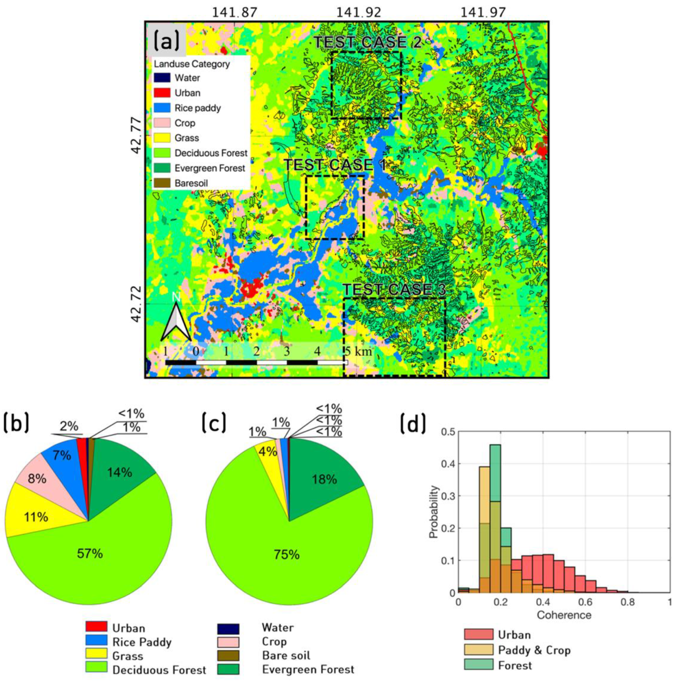
2. Hokkaido (Eastern Iburi) Landslides

On 6 September 2018, the M6.7 earthquake, with its epicenter located at 47.686 N, 141.929 E and a depth of 35 km, struck the Hokkaido prefecture, Japan. The powerful ground motion of the earthquake caused not only structural damage to buildings and liquefaction on the ground but also thousands of landslides [31,32] (Figure 1). Those landslides killed 41 people and buried a number of houses and buildings. Most of the landslides were caused by shallow failures and categorized as planar and spoon types [32]. In the southeastern part of the area, the deep-seated landslides of dip-slipping were found.
Investigation revealed that the earthquake-induced ground motion, precipitation of Typhoon Jebi, and geological setting jointly contributed to the massive number of landslides [32,33]. According to [33], ground motion played a fundamental role in the massive number of landslides. Ground motion show high-amplitude, low-frequency narrow band pulses that induce significant displacements and accelerations on natural slopes [34]. The earthquake can cause the slopes to be unstable by causing a loss of strength in the slope material. According to the Japan Meteorology Agency (JMA), the earthquake triggered sudden slope failures [35]. In addition, the basement of the study area is composed of Neogene sedimentary rocks and covered mostly with pumice layers with a thickness of 1.5 m. The surface layers are inter-bedded with the pumice and ash, with a thickness of 4–5 m [32]. The volcanic deposits are generally characterized as high mobility layer compared to non-volcanic deposits due to their differences in granularity, collapsibility and water content [35]. Further, the Typhoon Jebi passed over Japan a few days before the earthquake and its precipitation had reached approximately 100 mm for 3 days. The rapid increase in pore water pressure in the pumice of upper layers could have led to the reduction in the shear resistance and played a role in the mobility of the landslides [33].
Immediately following the landslides, the Geospatial Information Authority of Japan (GSI) acquired aerial imagery over the whole area affected by the landslides on 6, 11 and 12 September 2018. The images clearly show the landslide scarps and debris deposits. Further, they manually extracted the landslide area using visual inspection and released the polygon product on their website (Figure 1b). They found more than 6000 landslide scarps and 1000 associated debris deposits [32]. We used these products to evaluate the performance of the landslide detection algorithms explained in Section 3.

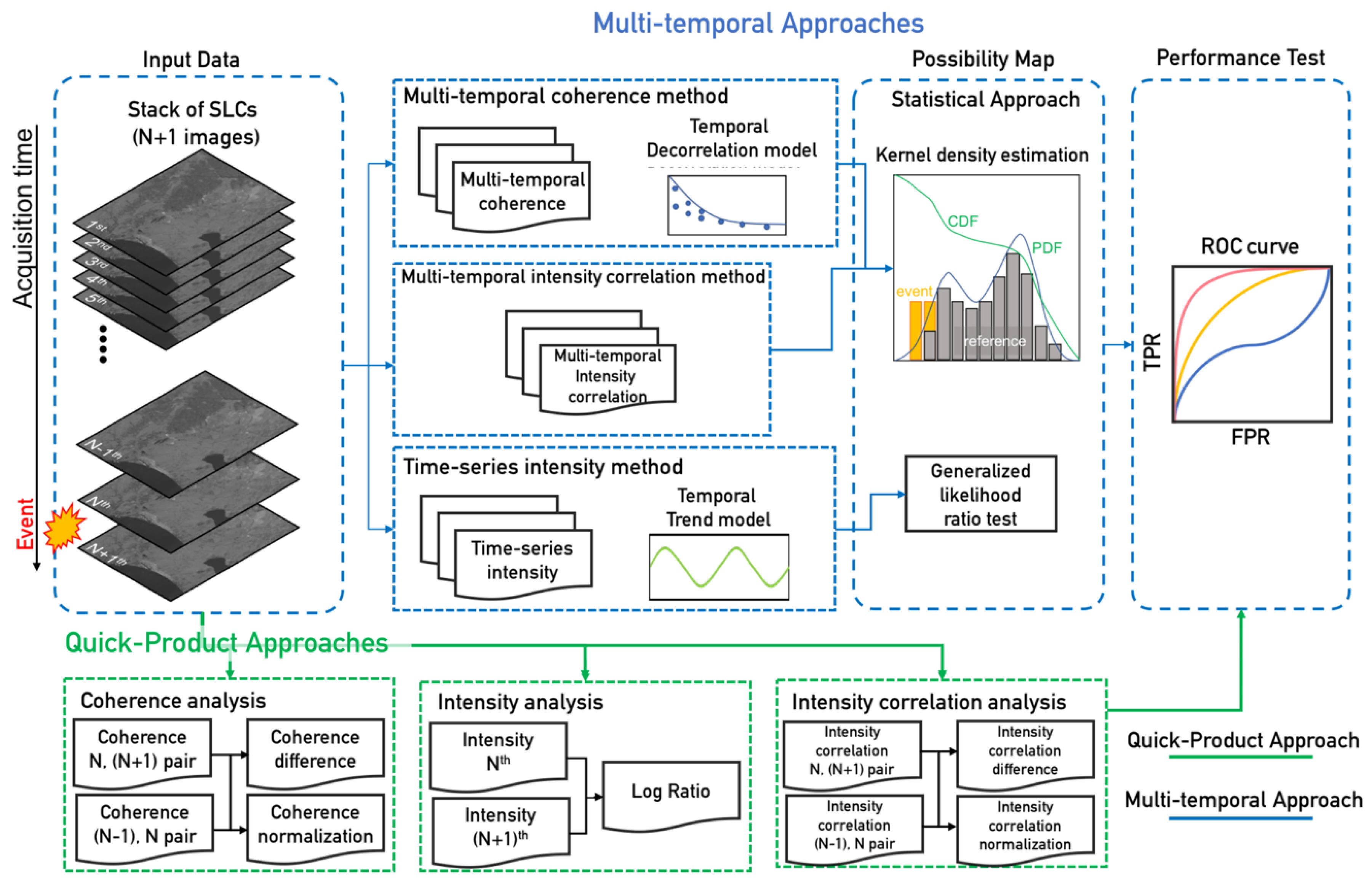
3. SAR data and Landslide Detection Methods

In order to detect landslides, we collected L-band ALOS2 PALSAR2 acquired from 11 January 2018 to 6 September 2018. The 17 scenes were acquired along the ascending orbit with left-looking and Ultra-Fine-Beam mode. Among the dataset, only the last image was acquired after the landslides. Their spatial resolutions are 3 m in range and 3 m in azimuth. The imagery was acquired with HH polarization and their incidence angles are approximately 43 degrees. All images are radiometrically calibrated and are co-registered using ISCE software [36,37,38].
If we have N + 1 SAR images assuming the major event occurs between image N and N + 1, then the complex reflectivity of the Single Look Complex (SLC) stack can be expressed as follows
X k = b ( k ) exp ( j θ ( k ) ) + n ( k ) k = 1 N + 1
where b and θ represent the amplitude and phase, respectively, and n is the zero-mean circular complex Gaussian random variable, with a standard deviation σ k . The backscattered power describes the interactions of the propagated electromagnetic wave with the scattering structure. Meanwhile, the phase θ is contributed from the scattering phase and distance between sensor and target including displacement, atmospheric phase delay, and topographic information. It is worth noting that the SLC stack has only one image acquired after the event, assuming the rapid response scenario.
In this study, we designed the landslide detection algorithms utilizing coherent and incoherent sources from the SLC stack to obtain the measure of changes. Coherence, intensity and intensity correlation are the representative measurements that have conventionally been used for change detection. Furthermore, we considered two scenarios depending on the number of available data: (1) a quick-product approach assuming a few images are available and (2) multi-temporal approach assuming we have enough numbers to analyze the temporal behavior as shown in Figure 2. Here, the quick-product scenario represents the comparison methods between the pre-event products and co-event or post-event products. In the case of the multi-temporal approach, we compared the reference group consisting of pre-event products to event groups consisting of co-event products.
To preserve the consistency of the spatial resolution of each method, we obtained the intensity value by multi-looking the SLC stack with 16 × 16 windows. Further, the coherences were estimated using the 16 × 16 multi-looked intensities and the 16 × 16 multi-looked interferograms. The intensity correlations were calculated from the 16 × 16 window.

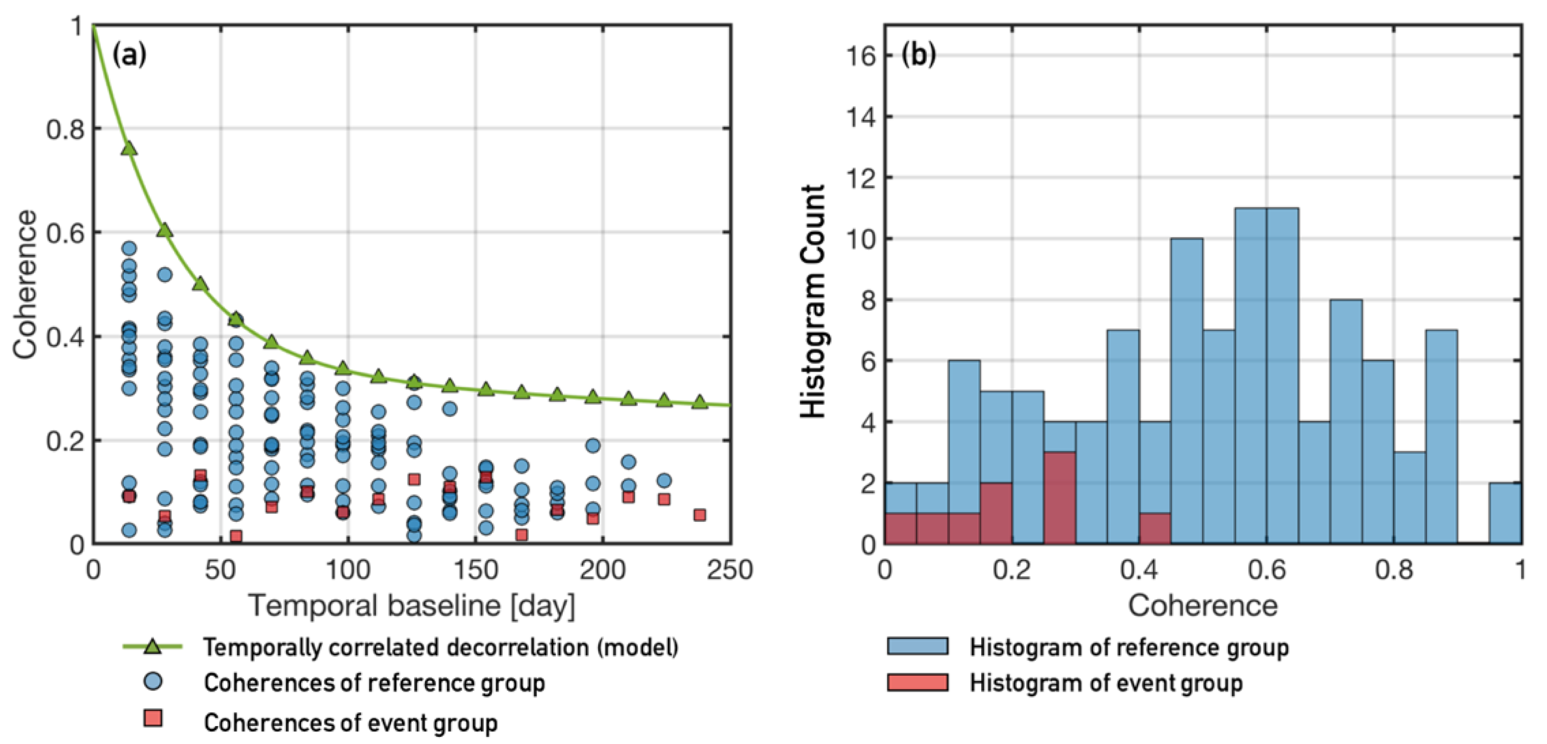
3.1. Coherence-Based Method

The complex coherence is defined as the correlation coefficient between two SAR scenes:
γ m , n = | E { X m X n e j φ m n } E { | X m | 2 } E { | X n | 2 } | m , n = 1 N + 1
where X m and X n denote the complex pixel values of mth and nth SAR scenes, respectively. We estimated the topographic phase and flat-earth phase, φ m n using from satellite orbits and Shuttle Radar Topography Mission (SRTM) digital elevation model (DEM) [39]. Thus, the coherence estimator of Equation (2) uses the phase of differential interferograms, which is correlated to displacement and atmospheric phase delay, to prevent the decorrelation caused by high fringe rate due to the steep slopes. Further, we used only the magnitude of coherence. In theory, the magnitude of the complex coherence is determined by the physical conditions of the scatterers, radar parameters, and the imaging geometry of the satellite. It is usually described as a product of four main components—geometric, thermal, volumetric, and temporal decorrelation [40]. Thermal decorrelation is a function of the SNR, which is related to the quality of the SAR imagery, and the backscattering characteristics responding to the electro-magnetic microwave. The geometric decorrelation is induced by the slightly different positions of satellites during the two acquisitions. The volumetric decorrelation is generally explained with the multiple scattering within volumetric targets due to the complexity of the scattering mechanism. The Random Volume over Ground (RVoG) model is one of the models to interpret the interferometric coherence observed over the forest target [41,42,43]. The temporal decorrelation is caused by changes (dielectric and/or structural properties) in targets on the ground. The abnormal signals from disaster events are directly related to the temporal decorrelation. Therefore, we exploit the characteristics of the temporal coherence.
Every change between the two acquisition times of the interferometric pair leads to the loss of coherence. In the case of the pair with the short temporal baseline (less than a few hours), the relocation of the scattering components in the pixel caused by the wind, especially in canopy, can lead to the decorrelation [44,45]. For the long temporal baseline (more than several days), the complexity of the natural changes including changes in the dielectric properties and location of the objects caused by rain, snow, wind, moving objects, etc., need to be taken into account [14]. Since the SAR imagery acquired at the satellite currently operating has a revisit time interval of several days, the scenario for the long temporal baseline needs to be considered. The changes caused by the major natural disaster is also one of the decorrelation sources.
In the aspect of the quick-product approach, the discrimination between decorrelations caused by natural disasters and natural phenomena can be achieved through the coherence difference, γ C D , and the coherence normalized difference, γ N C D , between the pre-event coherence and co-event coherence [5,9,46].
γ C D = γ N 1 , N γ N , N + 1
γ N C D = γ N 1 , N γ N , N + 1 γ N 1 , N + γ N , N + 1
These approaches have two assumptions: (1) the event-derived decorrelation is stronger than the nature-derived decorrelation and (2) the decorrelation of the natural phenomenon can be negligible or canceled out during the difference and ratio operator. In general, the identical temporal baselines for two pairs are required to safely satisfy the second assumption.
However, the second assumption may not be guaranteed for all cases, in particular for pixels with the objects easily affected by the natural changes. For example, the pre-event coherence may not be the representative value when temporal decorrelation caused by natural phenomenon is dominant. On this point, we can find why the multi-temporal coherence analysis is necessary because the historical behaviors to the natural changes can be exploited and the possibility can be estimated as to whether the decorrelation is caused by natural phenomena or by the major disaster.
Several kinds of literature have developed the multi-temporal coherence analysis by making a covariance matrix consisting of coherences for all interferometric combinations [11,14,28]. J. Jung et al. [11] introduced the multi-temporal coherent change detection method incorporating the temporal decorrelation model to interpret the temporal decorrelation patterns and isolate the contribution of natural disasters from the natural phenomena. [11,14] The temporal decorrelation model was designed from the basic frame of the RVoG model, which has volume and ground layers, by adding the temporal decorrelation terms as below.
γ = exp [ Δ T τ v ] γ t _ r a n d v + μ exp [ Δ T τ g ] γ t _ r a n d g 1 + μ
From the above equation, the temporal decorrelation model describes not only decreasing coherence with time intervals as shown as a green line in Figure 3a, as well as the random loss of coherence. The losses of the coherences with time intervals were modeled by the exponential functions with the temporal baseline Δ T . The terms, τ g and τ v , indicate the characteristics of time-correlated decreases for ground and volume layers, respectively. They are realistically assumed that the coherence of the volume layer is fast decayed and the ground layer remains relatively stable, i.e., τ g > τ v . The model also has the terms describing the random temporal changes that are not explained with the exponential decay function, namely temporally uncorrelated changes, i.e., γ t _ r a n d v and γ t _ r a n d g . Since the coherence is determined as the effective sum of the ground and volume layer contributions, the model has the ground-to-volume ratio, μ , to balance their contributions. The role of this model in terms of anomaly detection is that the event-derived decorrelation can be highlighted by estimating and detrending the time-dependent decaying coherence. As shown in Figure 3a,b, the decorrelation caused by the natural phenomena (blue circles in Figure 3a, and blue bars in Figure 3b can be characterized using the temporal decorrelation model and statistical histogram. Meanwhile, the strong phase disturbance caused by the natural hazards (red squares and red bar in Figure 3a,b respectively) drops the coherence to zero with the loss of the coherent signal. Therefore, abnormal behaviors over the time intervals can be isolated from the reference group and detected through the multi-temporal coherence analysis. The model parameter estimations were carried out with the least-regression methods [11].
The estimated model parameters are reintroduced into the estimation of the anomaly possibility map. The temporally uncorrelated terms indicate how the objects react to the natural changes without the exponentially decaying behavior. Thus, if a certain phenomenon strongly affects the object in the pixels, the method calculates the probability by comparing it with the historical decrease in the coherence. If the calculated probability is located near the middle of the histogram, it can be recognized as a casual phenomenon. In contrast, the probability is located at the end of the histogram, then one can guess the unusual phenomenon may occur (red histograms in Figure 3b). Therefore, the algorithm can isolate the landslide-induced signal from the natural-phenomenal signal based on the frequency and its strength observed from historical observations. Eventually, the multi-temporal methods can enhance the accuracy of landslide (anomaly) detection.
However, both the quick-product and multi-temporal approaches may fail when the observed coherence is always low independently with the time intervals. In this case, the observed coherence does not have the capability to detect the disaster-induced decorrelation because reference values are already close to zero. This behavior is often observed over flat surface areas such as water surface, road, etc., due to the low-returned signal as well as objects prone to decorrelation (ex. forest). Hence, the robustness of the coherence-based methods can be found over man-made structures such as houses and buildings because they have high SNRs and they are unlikely to be decorrelated even in long temporal baselines [47].

3.2. Amplitude-Based Method

In this study, the two different approaches are designed for the incoherent landslide detector, i.e., intensity analysis and intensity correlation analysis. From Equation (1), the intensity can be obtained as I k = | X k | 2 .

3.2.1. Intensity (Amplitude) Analysis

When two SAR images are obtained before and after the major event, the log-ratio of intensity is calculated as
I r a t i o = 10 · log 10 ( E { I N } E { I N + 1 } ) .
Since this method is simple and robust for a variety of cases, the log-ratio has been often implemented for many change or damage detection cases. The landslide detection using the log-ratio value is based on the basic assumption that landslides change the dielectric characteristics of the land cover. Depending on the property changes before and after the landslides, the log-ratio can be either positive or negative [24]. When the surface roughness increases as a result of the landslide, the backscatter signal increases, and the I r a t i o consequently decreases. In addition, since the moisture contents of the top layer of the surface soil have a positive correlation to the backscatter power, the changes in the soil moisture affect the log-ratio. Therefore, either positive or negative change can be recognized as a result of changes.
However, the log-ratio method using the pre-event and post-event scenes may lead to inaccurate results when the seasonal or natural phenomena prevail inducing the harmonic pattern of the time-series backscatter coefficient. For example, the dielectric characteristic changes by the seasonal precipitation trend could be a reason for false alarm [18]. Also, the growth and fall of the forest leaves, which is a volume scattering component, contribute to the total backscattering constant. Thus, the man-made or natural phenomena derive seasonal behavior or may be misinterpreted as the anomaly in the log-ratio analysis. In order to cope with this weakness, the multi-temporal analysis can be introduced. In this study, the multi-temporal intensity analysis is designed with two steps, which are the (1) temporal trends analysis and (2) multi-temporal assessment based on statistical distributions of intensity. In order to exploit the temporal trends, we modeled two major components, which are harmonic change and the temporally linear trend as following [48].
I o b e r v a t i o n ( t ) = I 0 ( t ) + i = 1 k ρ i s i n ( 2 π i t f + δ i ) + α t
where the second term describes the seasonal change and the third term is the linear trend. The pure signal without the temporal trend, I 0 , is the estimated value from observation, I o b e r v a t i o n , i.e., multi-temporal intensity. The harmonic change term consists of the amplitude of sine function, ρ i , the frequency, f , and phase δ i . The linear trend is simply determined by the slope of the time series, α . The number of cycles, k = n/2, is possible to estimate with the sampling frequency 1 / f . According to literature, in practice, a value of k = 3 has been found to be sufficient to model the temporal trend on the scale of approximately four months [18,48]. The coefficients can be estimated using the linear regression method for the time series. In order to avoid the impact of the disturbance caused by the major event, the regression processes are carried out with only the pre-event images.
After detrending and deseasonalizing the time-series intensity, we can successfully assume that the variation of the time-series intensity is governed by the statistical distribution of the intensity. According to the literature [49,50,51], the multi-looked intensity by averaging the L single-look intensity are described as the gamma distribution, as
p ( I 0 ) = 1 Γ ( L ) ( L λ ) L I 0 L 1 exp ( L I 0 λ )
where Γ ( · ) is the standard gamma function, L represents the equivalent number of looks and λ indicates mean intensity. In order to determine whether an arbitrary scene is changed by the natural disaster, or unchanged comparing the statistical distribution observed in pre-event images, we can apply the hypothesis test method. Let us assume that a null hypothesis, H o , indicates no change, and an alternative hypothesis, H 1 , represents change. For the multi-temporal approach based on the rapid response scenario, the joint probability density function can be formulated for the H o and H 1 .
p ( I 0 | H o ) = m = 1 N + 1 ( 1 Γ ( L ) ( L λ 1 ) L ( I m o ) L 1 exp ( L I m o λ 1 ) )
p ( I 0 | H 1 ) = m = 1 N ( 1 Γ ( L ) ( L λ 2 ) L ( I m o ) L 1 exp ( L I m o λ 2 ) ) · ( 1 Γ ( L ) ( L λ 3 ) L ( I N + 1 o ) L 1 exp ( L I N + 1 o λ 3 ) )
Here, the alternative hypothesis assumes that the intensity values have a gamma distribution without any changes before the Nth image, and that the changes occur for the N + 1 image. λ is given by the maximum likelihood estimates by averaging the time series of intensity values [50], i.e.,
λ 1 = m = 1 N + 1 I m o N + 1 , λ 2 = m = 1 N I m o N , λ 3 = I N + 1 o
Substituting Equation (11) into the probability density function (PDF), the generalized likelihood ratio test can be obtained as
Λ = p ( I 0 | H 0 ) p ( I 0 | H 1 ) = ( λ 3 ( λ 2 ) N ( λ 1 ) N + 1 ) L = ( I N + 1 o ( m = 1 N I m o N ) N ( m = 1 N + 1 I m o N + 1 ) N + 1 ) L
log Λ = L ( log λ 3 + N log λ 2 ( N + 1 ) log λ 1 )
When the intensity after the event, I N + 1 o , is perfectly identical to the averaged intensity value of images acquired before the event, Λ becomes 1. In contrast, the Λ is closer to zero as the I N + 1 o is more different to the normal status. It is worth noting that both positive and negative changes result in decreases in Λ .

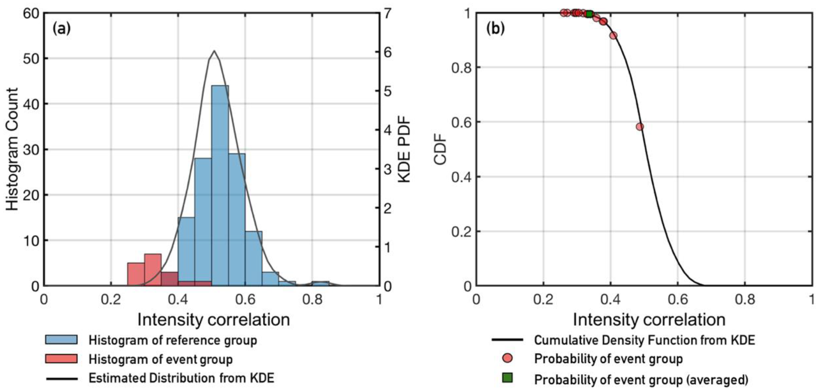
3.2.2. Intensity Correlation Analysis

Intensity correlation is a quantity to measure the correlation between two scenes over the given windows and is described as [52,53]
ρ m , n = E { ( I m I m ¯ ) ( I n I n ¯ ) } E { ( I m I m ¯ ) 2 } E { ( I n I n ¯ ) 2 } m , n = 1 N + 1
where I m and I n are two single-look intensity images. The intensity correlation identifies the changes in the textural modulation of the intensity measurement [52]. One may notice that the form of the formulation of the intensity correlation is similar to the coherence estimation (Equation (2)). Here, the difference between the intensity correlation and the coherence is that the coherence is determined with the changes in the phase. This difference enables us to detect the different range of the damages: the coherence may have the advantage to detect the subtle changes unseen through the optical imagery [26]. However, the coherence tends to be decorrelated when the scattering phase in a resolution cell is prone to the natural phenomenon. Therefore, the short temporal baseline is usually required to retrieve the reliable comparison of pre- and post-event coherence. On the other hand, the loss of the intensity correlation is related to the changes in the dielectric characteristics, which is the amplitude, not by the phase. Thus, the intensity correlation may have the possibility to still provide the change information even in the long temporal baseline.
Similar to the coherence-based methods, the landslide detection strategies based on intensity correlation can be designed when three SAR images are available. The difference, ρ I D , and normalization difference, ρ N I D , of the intensity correlation can be formulated as follows
ρ I D = ρ I r e ρ I c o
ρ N I D = ρ I r e ρ I c o ρ I r e + ρ I c o
When the multi-temporal SAR images are available, the intensity correlations can be obtained from the combination of pairs. Then, the multi-temporal intensity correlation measurements can be divided into the reference group, which consists of SAR images before the event, and co-event groups, which consists of the intensity correlations between SAR images before and after the event. The reference group involves the decorrelated signal caused by the natural and man-induced changes. One way to evaluate the possibility of landslides included in the event group is to compare the frequency and strength of the natural and man-induced decorrelations to the event group. It can be achieved by building the histogram of the reference group representing how often the strong decorrelation occurred before the event. Here, their effects are actually difficult to model, but, alternatively, we can estimate their behaviors using the kernel density estimation (KDE) method as shown in Figure 4a [54]. KDE is a statistical way to estimate unknown probability density function (PDF) by smoothing the finite and discrete samples. We estimated smoothed pdf using the KDE method for the reference group and we can convert it to cumulative density function (CDF). Then, we can estimate the position along the CDF line for the co-event group and obtain the possibility of landslides (anomalies) pixel by pixel (Figure 4b). If the positions of the event group along the CDF line are close to the end of PDF or 1 of CDF, this event group is assumed to show abnormal behavior, which has a high probability of landslide-affected area. Since the intensity correlations of the co-event group also have the undesired contributions, i.e., natural and man-induced signals, their effects can be mitigated by averaging the stack of possibility maps along the time axis.

4. Experimental Results

According to the land use map (Figure 5a) provided by Japan Aerospace Exploration Agency (JAXA) (https://www.eorc.jaxa.jp/ALOS/lulc/lulc_jindex.htm), the study area has a variety of land use-types including urban, paddy, crop, bare soil, grass, deciduous forest, and evergreen forest [55]. Figure 5b illustrates the portion of each category of land uses over the whole study area. The study area is mainly covered by forest including evergreen and deciduous forest (~71%). Further, 15% of the whole study area is used as the agricultural area including crop and rice paddy area. This observation indicates that most pixels over the study area are covered by the vegetation. We also investigated which land uses were mostly affected by the landslides. Here, approximately 93% of the destroyed and affected area by the landslides were mainly covered by the forest as shown in Figure 5c. Only 1% of the landslide-induced damage occurred over the houses. In order to understand the coherence characteristics of land uses, we averaged the pre-event coherences for each land use category. The average coherences of the forest area show relatively low values (~0.18). Thus, the detection capability over the low coherence area is a key factor to accurately detect landslides. We divided the whole area into three test cases (Figure 1a,b) and tested using the quick-product and multi-temporal approaches.

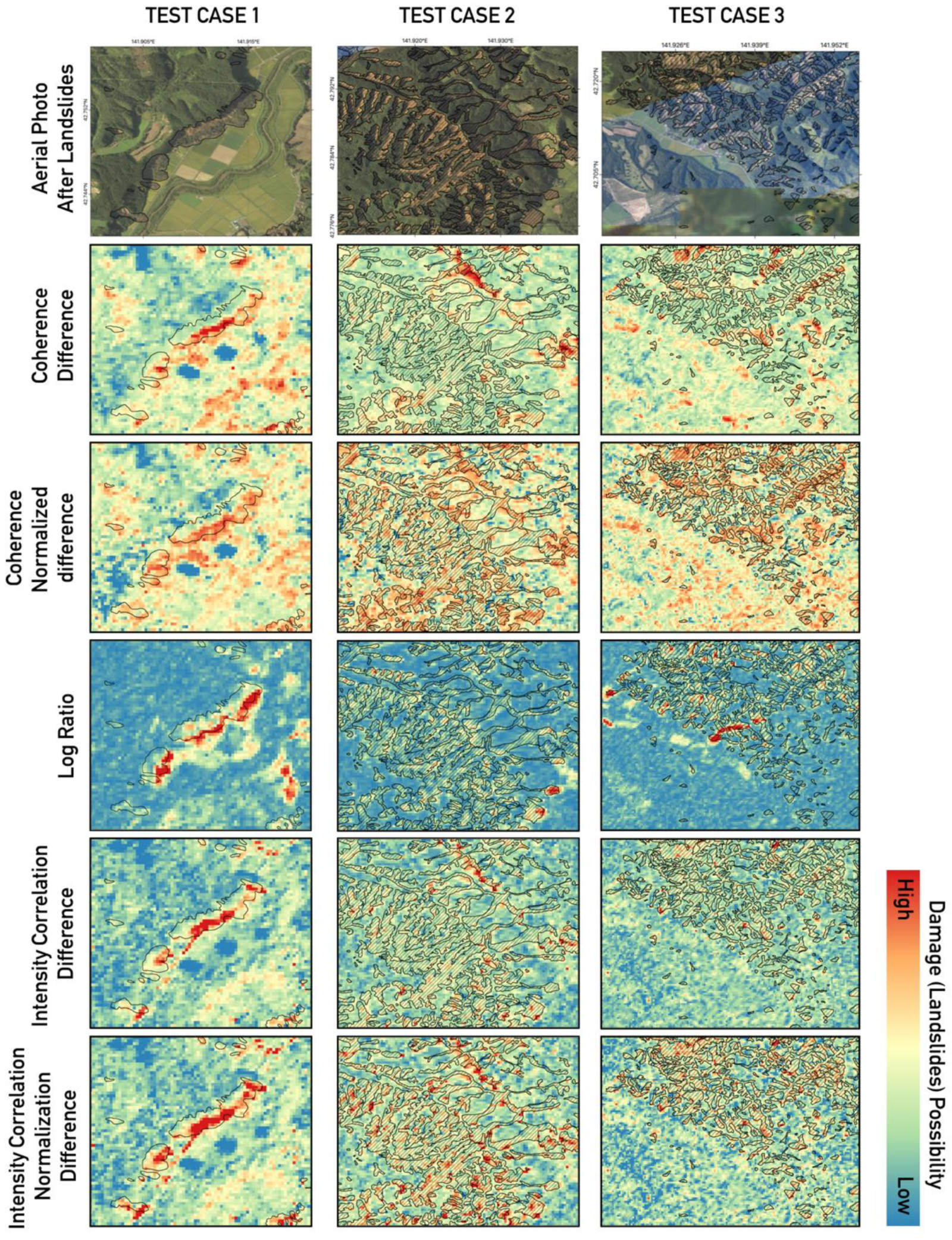
4.1. Quick-Product Analysis

First, we assume that the available data is limited. When only two images are available, acquired before and after the event, the log-ratio of the intensity can be applied. When the two images obtained before the event are available, we can test the difference and normalized difference for coherence and intensity correlation. In the log-ratio analysis, the images acquired on 23 August 2018 and 6 September 2018 were used as the pre- and post-event images, respectively. Further, the pre-event coherence and intensity correlation are calculated from images acquired on 9 August 2018 and 23 August 2018. The co-event coherence and intensity correlation are made using images acquired on 23 August 2018 and 6 September 2018. Hence, the temporal baselines of the pre-event and co-event are identically made using pairs with a 14 day time interval.
Figure 6 shows the results of the landslide detection algorithms for three test cases. The first test case represents an area where the landslide caused huge damage to houses, along the foot of hills, and over the parts of the crop area. The coherence difference and normalized difference of coherence show similar spatial patterns, with distinct signals over the houses. The difference between the two methods is that the coherence difference has a high level of false alarms over the crop area, while the coherence normalized difference has less noise. The log-ratio method shows the strong changes over the house, but also has a strong false alarm over the crop area. This implies the dielectric characteristic may change during the interval before and after the event. In comparison, between the log-ratio image and the coherence-based methods, the log-ratio method has relatively lower noise over the forest area. In test case 1, the intensity correlation difference and normalized difference have better performances over the crop area, with a similar performance for the houses in comparison with the other methods.
In the case of the forested regions (test case 2), the landslides are only observed through the log-ratio and intensity correlation. This implies that the landslides affected the dielectric characteristics or/and surface roughness, and the incoherent methods are capable of detecting them. The coherence-based methods show the noise and high false alarm rate. As a result, the coherence-based method does not provide useful information on this case of the landslide.
The third case is covered by 12% of the crop area and 88% of the forest. The results are identical to the second case, meaning that the intensity correlation and log-ratio methods detected the landslide signals over the forest region. In comparison, between the difference and normalized difference of intensity correlation, the normalized difference of intensity correlation depicted the higher values over the landslide area. However, both detectors show the intermediate level of the landslides possibility over the crop area, which represents that the changes over the crop area are being recognized as the landslides. Unfortunately, we were not able to see the clear signal of the landslides though the coherence-based methods. The normalized difference of the coherence seems to better detect landslides but it also shows high false alarms over the crop area as well. The coherence difference only depicts the intermediate level of the possibility over landslides and crop areas.
Since the test cases 1–3 consist of many objects with diverse characteristics, the observation from test cases shows some insights on how the landslide detections using coherence, intensity, and intensity correlation perform for the different land uses. Overall, the coherence-based methods are capable of detecting the landslides over the human-made structures as shown in test case 1. However, they may poorly work over the forest area as test cases 2 and 3. This proves that the decorrelation caused by natural phenomena can lead to significant decorrelation and also severely affect the detection performance. The log-ratio has the capability to find landslides over the forest, implying that the landslides affected the dielectric characteristics and/or surface roughness. However, this property may contribute to false alarms over crop areas where the backscattering changes as well. Interestingly, the intensity correlation methods are not significantly affected by the strength of the backscatter signal, showing the relatively low level of landslide possibility over the crop area. Therefore, in the case of the quick-product analysis, the intensity correlation-based methods can be robust for the heterogeneous area including human-made structures and forest regions. We will discuss the quantitative performance of each detector more in Section 4.3.
It is also worth noting that the normalized difference is usually better than the simple difference. This is because the normalization process adjusts difference values to a notionally common scale. Let us assume that we observe coherence drops at the two independent pixels with an intermediate and high coherence of pre-event pair. Even though the two pixels are identically affected, the simple difference method could show more changes on the pixel with high coherence (e.g., 0.5 → 0.1 ≥ 0.4 vs. 0.9 → 0.1 ≥ 0.8). Meanwhile, the normalization adjusts the difference based on the sum of the pre- and co-event values, and then it eliminates the effects of certain gross influences (e.g., 0.5 → 0.1 ≥ 0.67 vs. 0.9 → 0.1 ≥ 0.8). Therefore, the normalization could be more beneficial for change detection.

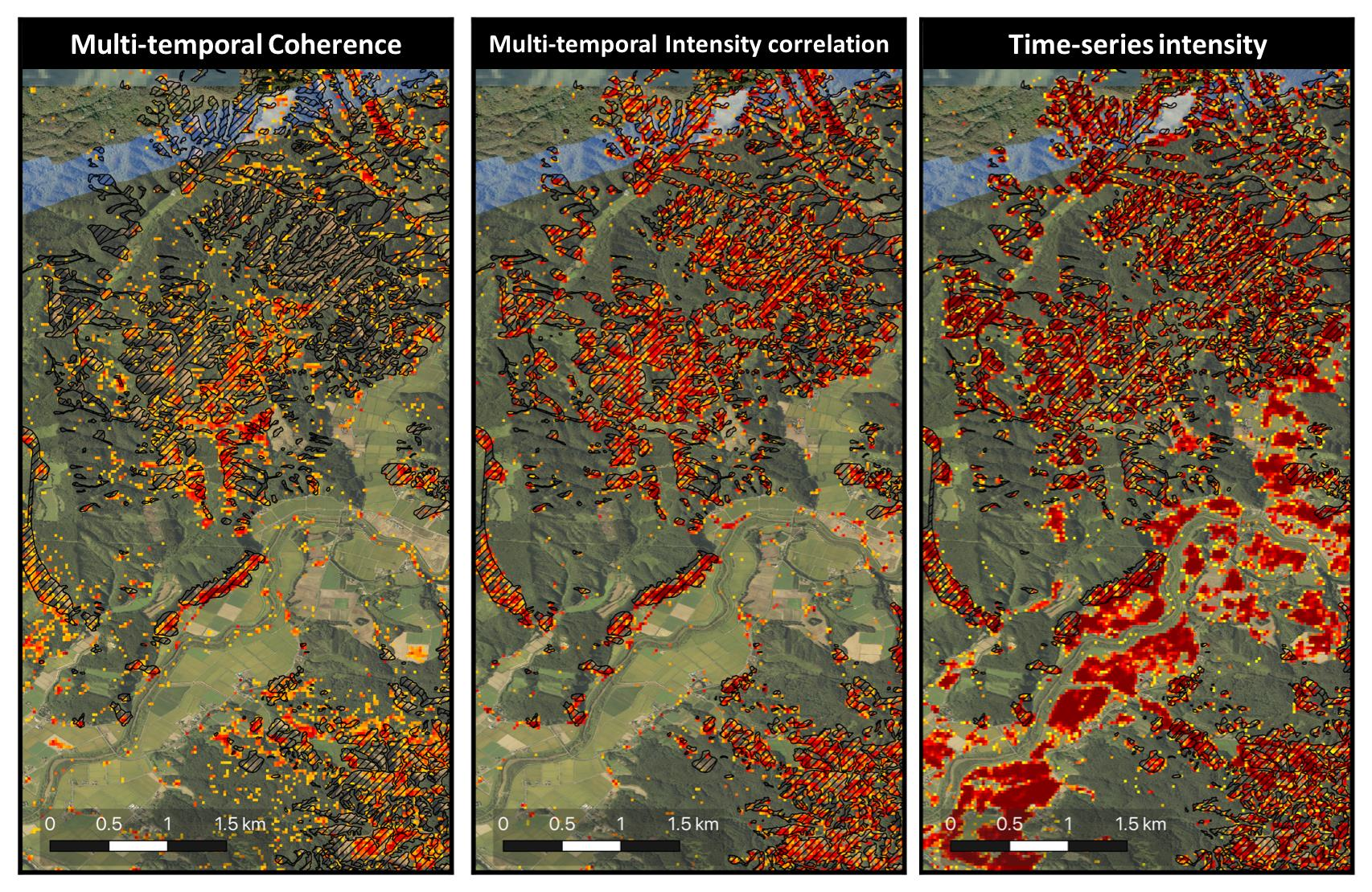
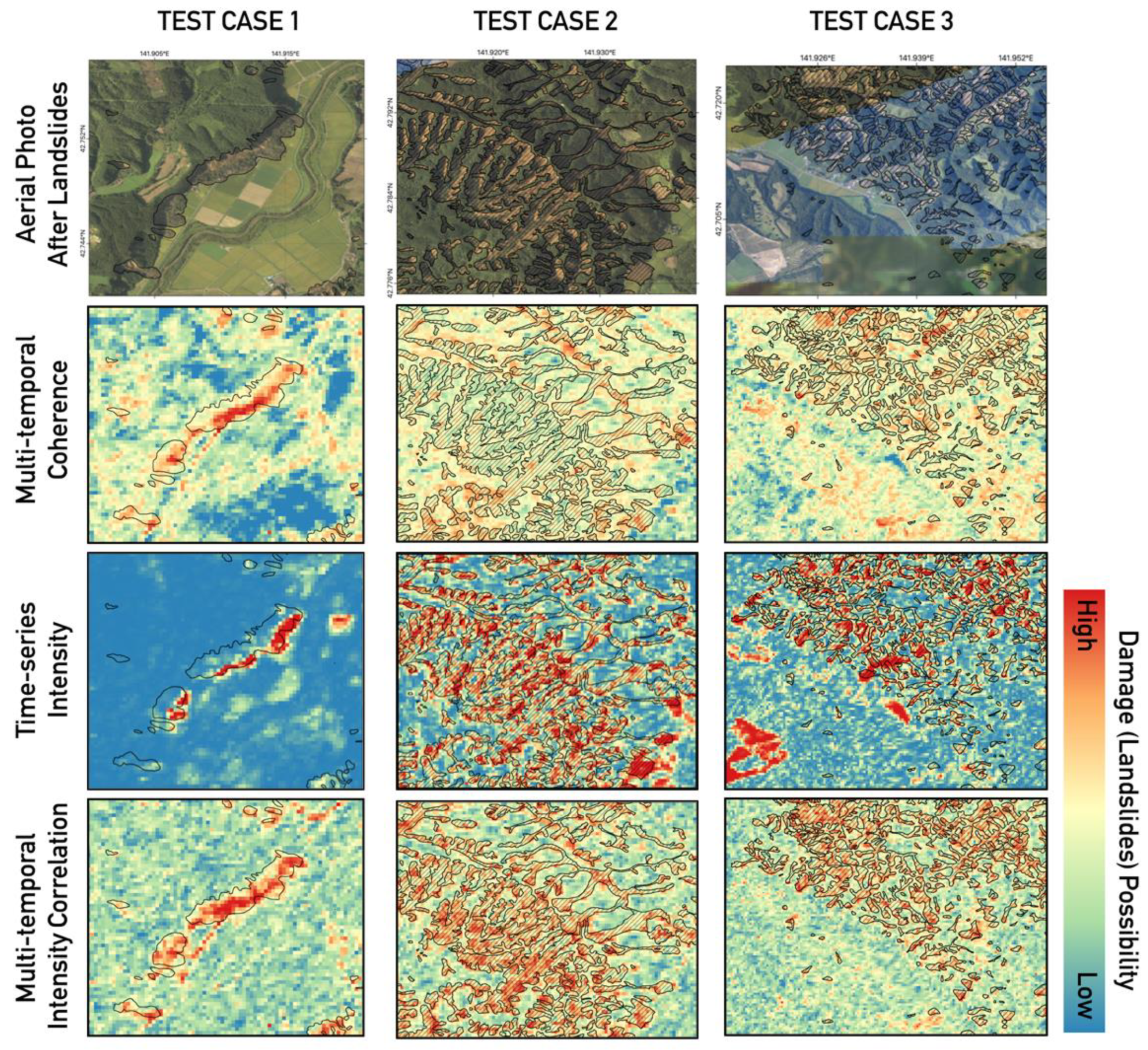
4.2. Multi-Temporal Analysis

In the case of the multi-temporal analysis (more than three images), the approaches are designed to detect the abnormal signal in comparison with the reference (pre-event) images. Hence, as introduced in Section 3, we grouped the pre-event coherences/intensity correlations obtained from the pair-wise combinations as the reference group. Meanwhile, the co-event group consists of coherence/intensity correlation made from the images acquired before the event and one image after the event. Thus, the reference group has 120 coherences/intensity correlations, and the co-event group has 16 coherences/intensity correlations. We used all coherences and intensity correlations for the multi-temporal coherence and multi-temporal intensity correlation methods, respectively. Unlike the multi-temporal coherence/intensity correlation methods, time-series intensity analysis uses each scene as inputs of the algorithm. Therefore, only one intensity image is the post-event group and 16 pre-event images are involved in the reference group.
Figure 7 illustrated their results. We found that the multi-temporal methods overall produce more accurate detection results in comparison with the quick-product methods. In test case 1, the multi-temporal coherence reduces false alarms over the non-landslide area. However, it shows a high probability over the landslide areas. However, the multi-temporal coherence method still has a similar level of accuracy over the forest area in comparison with the quick-product approaches as shown in test cases 2 and 3. Based on the visual interpretation, it is revealed that the time-series intensity analysis slightly improves the performance compared to the log-ratio technique for the second and third cases. However, the time-series approach even worsens the accuracy over the crop area due to the abnormal signal of crop area. The multi-temporal intensity correlation approach is proven as the most reliable detector. It not only gives lower false alarms over the crop and forest area comparing the quick-approach of the intensity correlation but also most agrees with the polygons of landslides among the approaches.
From the test cases 1–3, we were able to see how the multi-temporal detectors work for different land uses. Similar to quick-product analysis, the multi-temporal coherence and intensity correlation method produced well-matched results with the polygon embedding the human-made structures, as shown in first test case. This finding indicates pixels, where the human-made structures are located, have stable and reliable coherence and intensity correlation values before the landslides. Further, it represents that the landslides dropped significantly drop the coherence and intensity correlation. However, the time-series intensity did not work very well in the test case 1. This may indicate the backscattering change was not enough large to be detected.
As revealed in test case 2 and 3, the landslides affected the backscattering characteristics over the forest. Accordingly, the time-series intensity and multi-temporal intensity correlation approaches are capable of detecting the landslides and resulting in the relatively reliable performances over the forest area. These results are distinguishable from the multi-temporal coherence analysis which poorly worked for the forest area due to the decorrelation of the reference group. This finding seems related to the characteristics of measurements. Since coherence usually is too sensitive to the temporal changes induced by natural phenomena, the temporal baseline can play a key role in the performance of change detection. The unsuccessful detection performance of the multi-temporal coherence may represent the 14 days repeat-pass cycle is not temporal sampling to obtain reliable temporal behaviors of forest over our study area. In contrast, since the multi-temporal methods employing the amplitude are less affected by the temporal baseline, they still have the potentials to monitor the change over the forest.
Interestingly, the performance of the time-series intensity analysis over the crop area seems unsuccessful as shown in test cases 1 and 3. As consistently shown in the quick-product approach, the relatively strong changes in backscattering intensity seem to be observed and result in the increase in false alarms. At this point, we can differentiate the time-series intensity and multi-temporal intensity correlation method. The intensity correlation is related to the texture variation over the observation period rather than the backscatter value, unlike the time-series intensity analysis. This is why the intensity correlation has better performance over the agricultural area.
Based on the finding of three test cases, we can extend our expectation to the entire area. Since the Area Of Interest (AOI) mainy consists of forest and agricultural area, we can expect the multi-temporal intensity would be a most powerful detector for the Hokkaido landslide. More detailed analysis will be explained in Section 4.4.

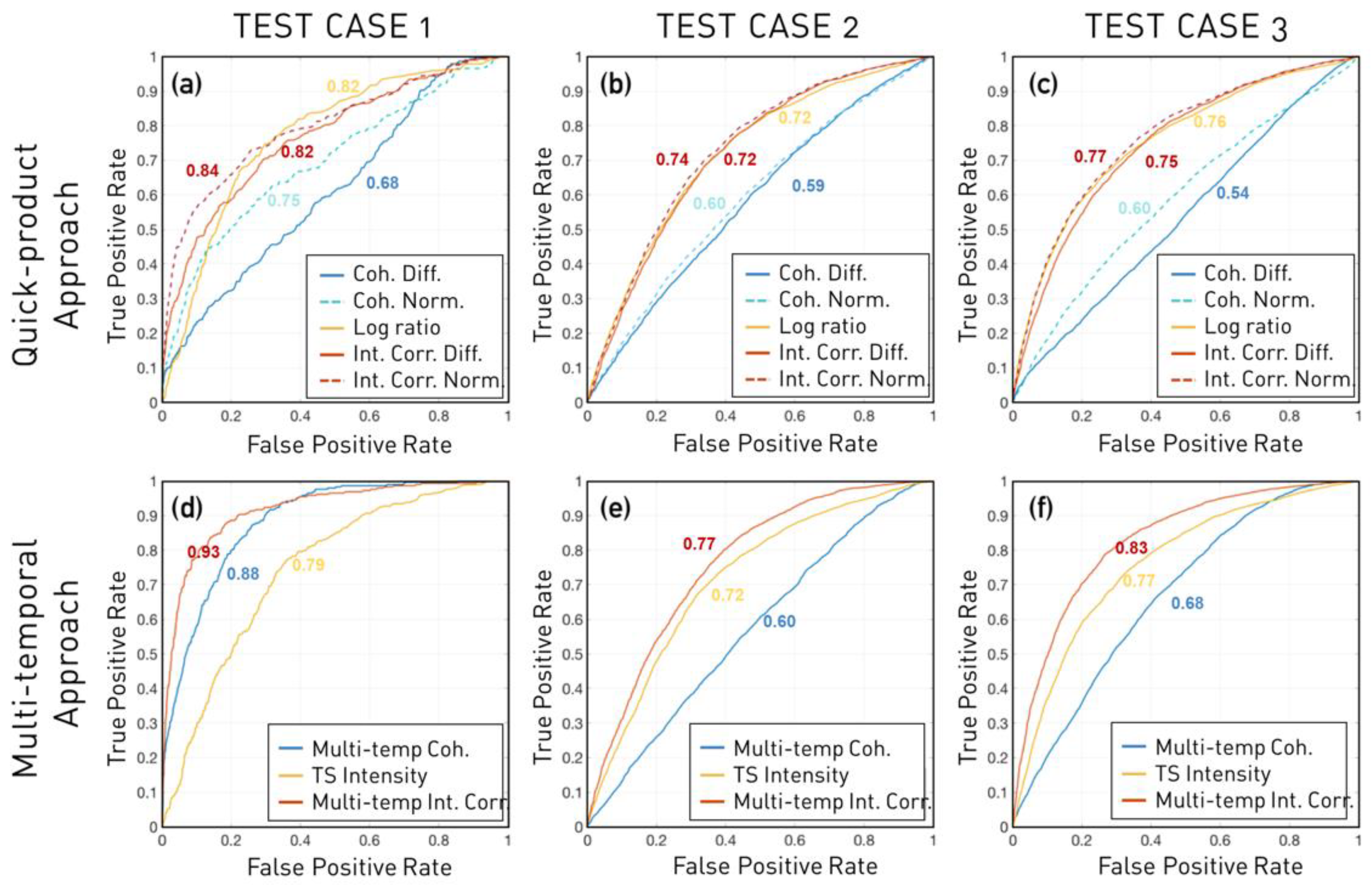
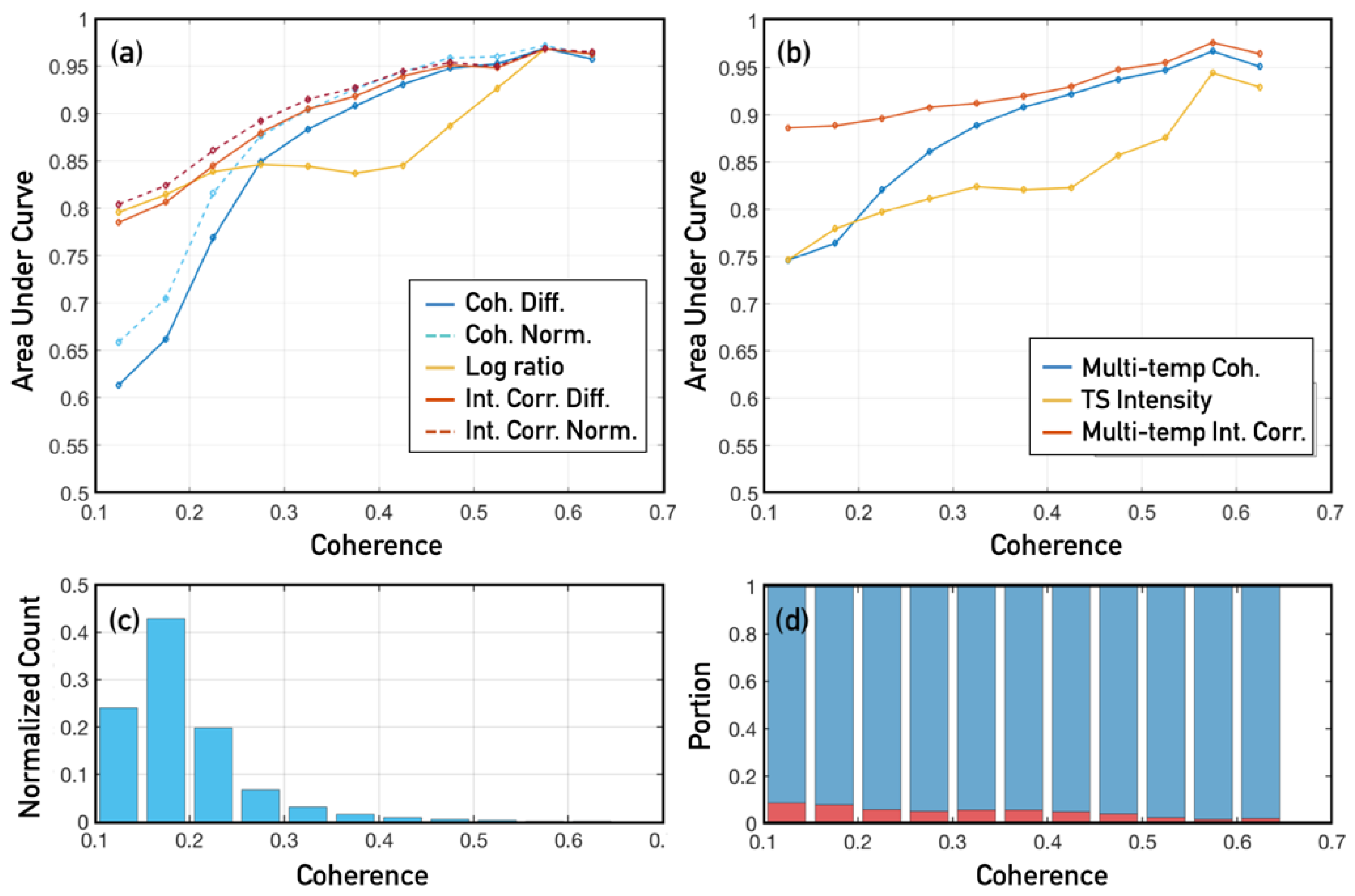
4.3. Performance Test Using ROC Curve Analysis

Receiver Operating Characteristic (ROC) curves enable us to quantitatively analyze which detection algorithms are capable of detecting the changes against the false positive rate at various discrimination threshold settings. This analyzer can be more suitable to test the performance of the method, resulting in the continuous values as our results rather than the binary classifier, by calculating trade-off between the true positive rate (TPR) and the false positive rate (FPR) with the arbitrary thresholds. From the ROC curve, it is also possible to calculate the Area Under the Curve (AUC) as a measure of aggregated detection performance. The 0.5 of AUC represents that the algorithm does not have the ability to detect the change and 1 of AUC indicates the perfect delineating the landslides. The ROC curves were illustrated in Figure 8 for three test cases using the quick-product approach and multi-temporal approaches.
Depending on the portion of land uses for each case, the ROC curves of each detector show different levels of TPR as the FPR increases, because the scatterers belonging to each category of land uses differently react to the natural disaster and natural phenomena. In the case of the quick-product approaches, the normalized difference of intensity correlation shows the best performances among the methods. We found its AUCs for the three cases are 0.84, 0.74, and 0.77, respectively. Interestingly, the log-ratio method seems to have a slightly lower performance compared to the intensity correlation methods, but still provides meaningful AUCs, showing 0.82, 0.72, and 0.76 for three cases, repectively. In contrast, for our test cases 2 and 3, the coherence-based methods seem not to provide reliable information about landslides over the forest area. As listed in Table 1, the AUCs of coherence-based methods range from 0.58 to 0.6, meaning that these detection algorithms have poor capabilities to discriminate the decorrelations caused by the natural disaster from the natural phenomena over the forest area. In our analysis, the coherence-based methods are only reliable when the pixels have a relatively high coherences as the test area 1 in which the high coherence is observed due to the artificial structure such as houses. In comparison to the other detection algorithms, we found that the coherence-based methods were relatively less powerful. As a result, the delineating only the landslides may be difficult through the coherence-based methods over the forest area.
Among the multi-temporal approaches, the multi-temporal coherence methods dramatically increase the performance compared to the quick-product coherence-methods for test case 1. However, it still suffers from the ambiguity between the decorrelation caused by the natural phenomena and landslides, resulting in the low performance, i.e.,0.58–0.67 over test cases 2 and 3, as shown in Figure 8d, and Table 1. It is worth noting that the time-series intensity method does not significantly impact the performance in comparison with log-ratio method. In contrast, the multi-temporal intensity correlation method improves the performance from the quick-products of intensity correlation methods leading to the most robust method as shown in Figure 8f and Table 1.
In order to quantify the performance of the detectors as a function of the coherence, we reanalyzed the ROC curve analysis with the different levels of coherence. First, we average the pre-event coherences to generalize the characteristics of each pixel. Then, we grouped the pixels with the coherence level ranging from 0.1 to 0.6 with the steps of 0.05. We carried out the ROC curve analysis and calculated corresponding AUC for each step. We plotted the diagnostic ability as a function of the coherence for the landslide detection algorithms as shown in Figure 9.
As shown in Figure 9a, the coherence-based methods show a monotonic increase as the coherence level increases. This observation implies that the coherence-based methods are more reliable at the higher coherence. However, it has severe drawbacks in low-coherence areas. In this study area, the observed coherence over the forest area was approximately 0.18 as shown in Figure 5d and 71% of land cover is forest. This is why the coherence-based methods poorly detect landslides. The AUC of the log-ratio test increases in the range of 0.1 to 0.25 of coherence level, decreases in the range of 0.25 to 0.45 and again increases over 0.45. It is worth noting that the log-ratio method better detects the disturbance for the low-coherence pixels, and also less affected by the coherence level. Interestingly, the intensity correlation methods tend to have better performance for the higher coherence group as similar to the coherence-based techniques. However, the intensity correlation shows the overwhelmed performance comparing with the coherence-based and log-ratio techniques.
The AUCs of the multi-temporal approaches are also compared with the quick-product analysis as shown in Figure 9b. The multi-temporal approaches except the time-series intensity analysis result in the higher accuracy over the low coherence as well as the high coherence. It is worth noting that the multi-temporal intensity correlation approach produced the highest AUC over the whole coherence level. In contrast, the multi-temporal intensity approach does not significantly improve the accuracy compared with the log-ratio test.
The ROC curve analysis for three test cases shows that the coherence-based methods including quick-product and multi-temporal approaches may be unsuccessful to detect the meaningful signal as shown in Figure 8 and Table 1. However, the analysis between the coherence level and AUC (Figure 9) provides another aspect of the potential of coherence-based methods. More precisely, the AUCs are larger than 0.9 for the pixels with the average coherence more than 0.35 as shown in Figure 9a. This finding shows that the coherence-based methods still have great potential for the intermediate- and high-coherence region. One may question why the coherence-based detectors poorly operated for the three test cases. The answer can be found in the pixel number of high coherence. As illustrated in Figure 9c, more than 90% of the pixels are concentrated on the coherence below 0.3. Hence, the poor performance of the coherence-based detectors over the low coherence level is affecting the test case analysis, as shown in Figure 8. Therefore, it would be difficult to identify the robustness of the coherence-based method in these test cases. In addition, the performance of the intensity correlation methods, in particular, multi-temporal intensity correlation, seem better than the coherence-based methods. However, one needs to pay attention to the number of pixels with high coherence, and the portion of the landslide and non-landslide areas (Figure 9d). Only ~2% of the pixels have a coherence over the 0.4 and the landslide areas are less than 8%. Therefore, the comparison between the intensity correlation and coherence-based methods for high-coherence regions could be a hasty generalization. Here, the most distinct finding seems, from our study, that the multi-temporal intensity correlation method gives very good results, even for very weak coherences, and is close to 1 as soon as the coherence is greater than 0.5. In addition, it also seems to work very well in forest areas.

4.4. Overall Accuracy Comparison

From the experimental results, we observed that the log-ratio has relatively low performance in comparison with the intensity correlation methods. Moreover, the time-series intensity method is sometimes worse than the quality of the results from the log-ratio test. For further clarification, we produced the landslide detection maps depicting the landslides and non-landslide areas using the thresholds corresponding to 0.2 of the false positive rate for each algorithm (Figure 10). Then, we calculated the overall accuracy metric for the two types of land uses, i.e.,rice paddy and crop and forest area. The overall accuracy (OA) is calculated as
OA = TP + TN TP + TN + FP + FN
where TP, TN FP, and FN are true positive, true negative, false positive, and false negative, respectively. The overall accuracy is listed in Table 2. We found that the multi-temporal coherence and intensity correlation methods have good accuracies over the rice paddy and crop area. In contrast, the accuracies of the log-ratio and time-series intensity correlation are severely lower than the other methods. The log-ratio method assumes that an area unaffected by the natural disaster has a similar level of intensity values to the pre-event image. However, the changes in the dielectric characteristics and surface roughness caused by agricultural activities including irrigation, drainage, and harvest induce the variation of the intensity values. Further, the heavy precipitation of the typhoon Jebi can be another reason to modulate the intensity. This reason can be also applied to time-series intensity methods. Hence, the GRLT method assumes no changes over the observation period before the event. When the variation of intensity is not fully modeled by the temporal trend model (Equation (7)), the assumption does not hold. In addition, when unpredicted natural phenomena, but not related to natural disasters, happen before the post-event scene, it may be recognized as changed. Hence, its underlying assumption might not be valid for the long-term time series for the crop area. Accordingly, the intensity variation before the target landslide would lead to inaccurate performance over the whole range of coherence levels.
In comparison, between the binary images of the time-series intensity and multi-temporal intensity correlation methods, as shown in Figure 10, the time-series intensity tends to highlight the backscattering changes over the crop area. This is because the time-series intensity estimates the changes in backscattering signals themselves. Meanwhile, the intensity correlation estimates the changes in texture rather than the amplitude of signals.
Another point we need to clarify in this paper is that the multi-temporal intensity correlation method is more reliable than the multi-temporal coherence approaches over the forest area. This is because the coherence of the forest is easily decorrelated due to the relocation of the scatterer inducing the phase disturbance. Further, the change in the dielectric characteristics of the ground layer and volume layer could induce the phase disturbance by changing the scattering phase center. In contrast, the intensity correlation could survive even in the strong wind unless the texture variation over the estimation window changes. Figure 11 shows the comparison between the coherence matrix and intensity correlation matrix derived from all interferometric combinations for the landslide pixel. We can clearly see the decorrelation signal at the last epoch for both matrixes (Figure 11a,b) when the average coherence is 0.47. However, it is almost impossible to distinguish the changes in the coherence matrix with low coherence (0.12). Meanwhile, there is still a possibility to observe the decorrelation through the intensity correlation matrix. Therefore, the intensity correlation methods could be complement detectors for low coherence area.

5. Discussion

The purpose of this paper was to investigate the potentials of the change detection algorithms based on coherence, intensity, and intensity correlation calculated from SAR images. These evaluations were carried out assuming circumstances when data availability is limited and multi-temporal data is available. To date, various studies using SAR imagery for landslide detection have been proposed. Many researches found that the amplitude difference and intensity correlation can be more practical and effective tools rather than coherence methods because of mountainous forest area and its severe decorrelation [23,24,25,56]. Moreover, [23] concluded that the intensity correlation could be better than the amplitude difference by investigating a landslide event on Kii Peninsula, Japan using two SAR images. Even though they used the single intensity correlation and we used two intensity correlations, this finding is consistent with our results. In addition, we compared the simple difference and normalized difference of the intensity correlation and found that the latter is better than the former.
Another noteworthy point in our paper is that multi-temporal analysis can improve the landslide detection accuries. We were not able to directly compare our study with other research due to the lack of case studies for the landslides. However, we definitely found the multi-temporal analysis can have a higher potential for landslide detection than quick-product analysis through the ROC curve and overall accuracy for diverse land uses. This benefit comes from the capability to discriminate against the natural hazards from the natural phenomena by statistically analyzing the normal status of each scatterer. Here, we can find the novelty and strength of our research.
The multi-temporal algorithms we developed have different performances for landslides that occurred over the diverse land uses. The multi-temporal coherence worked well for the human-made structures with high coherence. Meanwhile, the time-series intensity method shows a good agreement with the landslide polygons over the forest area but has poorly worked for the agricultural area. Interestingly, the multi-temporal intensity correlation method shows good enough to be applied to a variety of cases. Here, due to the lack of a sufficient amount of the high-coherence pixels, we were not able to carry out the profound and depth-in comparison analysis. According to [14], they proved the multi-temporal coherence analysis can provide a reliable burnt area caused by wildfire over the forest area. This shows that the performance of the multi-temporal coherence is more related to the coherence level rather than land use type. Therefore, the multi-temporal coherence may be applied for the landslide detection if the intermediate- or high-level coherence of the reference group is guaranteed.
For accurate performance analysis, the geometric distortion of the SAR image also needs to be considered. Two major distortions could affect the quality of landslide detection. First is the shadow region, where the radar signal cannot illuminate behind slopes because of the incidence angle and slope angle in the mountain area, and second is the layover region, where the top of a reflecting object is closer than the lower part to the radar. We generated a shadow/layover map from SRTM 30 m data, but found that our AOI does not have such effects.

6. Conclusions

This paper designed and evaluated landslide mapping algorithms using SAR images based on coherence and intensity information. For the rapid response scenario, the frameworks were divided into two cases, i.e., quick-product analysis and multi-temporal analysis. We adopted the conventional algorithms such as the coherence difference, normalized difference of coherence, log-ratio, intensity correlation difference, and normalized difference of intensity correlation for quick-product analysis. In the case of multi-temporal analysis, we developed and designed novel methods to differentiate the abnormal signals against the normal status by statistically analyzing the history of multi-temporal reference measurements. We carried out these algorithms for the Hokkaido landslides detection using L-band ALOS2 PALSAR2 images.
Our investigation reveals that the CCD may be unreliable when the coherences of the pre-event pair or reference group are not high enough. However, CCD worked well for the intermediate- and high-coherence regions. Further, we found that multi-temporal coherence analysis enhances the landslides detection performance. The log-ratio of intensity and time-series intensity methods proved their capability of landslide detection over the forest but may produce high false alarm over agricultural. Unlike the coherence-based methods, the intensity correlation methods seem to more accurately discriminate the landslide and non-landslide areas. Similar to the quick-product analysis, the multi-temporal intensity correlation method better distinguishes the landslide area from the non-landslide areas than the multi-temporal coherence method for all conditions of coherences. Besides, the multi-temporal approach improved the detection accuracy by reducing the false alarm rate compared to the difference and normalization of the intensity correlation. This finding implies that the intensity correlation methods can alternatively be used for the low-coherence region when the coherence is too low. Further, we were able to find high potential in the multi-temporal approaches to delineate the landslides.
In general, several considerations should be taken into account for the accurate detection of damages including landslides using SAR images. For instance, different types of natural disasters cause different levels of damage severities. Further, the successful delineation of the damages for a variety of cases is determined with the response of scatterer to radar signal before and after natural disasters. Thus, the types of changes as well as the characteristics of scatterers regarding the amplitude and coherence should be considered for the damage and change assessment analysis. Here, the Hokkaido landslides produced immense damage, turning the forest into bare soil, and the coherence was too low to generalize and obtain the characteristics before the event. Therefore, the performance of the change detection algorithms we tested may not be identical to the different cases. For example, the coherence-based methods could be better than the intensity based algorithms for the damage to urban areas as the other literature investigated. Therefore, compressive analysis and scenarios are prepared and need to be performed in order to rapidly respond to the natural disasters.
In this research, we tested the coherence, intensity, and intensity correlation independently. However, it is also possible to combine their workflows to improve accuracy. Since the data used in this experiment has single polarization, we were not able to study the advantage of additional polarizations such as dual-or full-polarization. Therefore, further research is needed for other SAR images, such as Sentinel-1, UAVSAR, and NISAR.

Author Contributions

Conceptualization, J.J. and S.-H.Y.; methodology, J.J.; software, J.J.; data curation, J.J and S.-H.Y; validation, J.J.; formal analysis, J.J. and S.-H.Y.; investigation, J.J. and S.-H.Y.; writing—original draft preparation, J.J.; writing—review and editing, J.J. and S.-H.Y.; visualization, J.J.; supervision, S.-H.Y.; project administration, S.-H.Y.; funding acquisition, S.-H.Y. All authors have read and agreed to the published version of the manuscript.

Funding

This research was sponsored by the NASA Earth Science Disasters Program and performed at the Jet Propulsion Laboratory, California Institute of Technology.

Acknowledgments

Original ALOS-2 data and products are copyright JAXA and provided under JAXA ALOS Research Announcement RA6. The authors would like to thank the GSI for providing aerial photos and detailed landslide extent polygons.

Conflicts of Interest

The authors declare no conflict of interest.

References

  1. Chen, Y.; Remy, D.; Froger, J.-L.; Peltier, A.; Villeneuve, N.; Darrozes, J.; Perfettini, H.; Bonvalot, S. Long-term ground displacement observations using InSAR and GNSS at Piton de la Fournaise volcano between 2009 and 2014. Remote Sens. Environ. 2017, 194, 230–247. [Google Scholar] [CrossRef]
  2. García-Davalillo, J.C.; Herrera, G.; Notti, D.; Strozzi, T.; Álvarez-Fernández, I.J.L. DInSAR analysis of ALOS PALSAR images for the assessment of very slow landslides: The Tena Valley case study. Landslides 2014, 11, 225–246. [Google Scholar] [CrossRef]
  3. Tuan, N.A.; Marianne, S.; José, D.; Marc, O.; Gerardo, H.G.; Carlos, G.L.-D.J.; Celestino, G.N.; Inmaculada, Á.F.; Bernard, M.; Joaquim, M.D.P. Spatio-temporal evolution of Ground displacement of the Tena landslide (Spain). In Landslide Science and Practice; Springer: Berlin/Heidelberg, Germany, 2013; pp. 133–140. [Google Scholar]
  4. Jia, H.; Zhang, H.; Liu, L.; Liu, G.J.R.S. Landslide Deformation Monitoring by Adaptive Distributed Scatterer Interferometric Synthetic Aperture Radar. Remote Sens. 2019, 11, 2273. [Google Scholar] [CrossRef] [Green Version]
  5. Yonezawa, C.; Takeuchi, S. Decorrelation of SAR data by urban damages caused by the 1995 Hyogoken-nanbu earthquake. Int. J. Remote Sens. 2001, 22, 1585–1600. [Google Scholar] [CrossRef]
  6. Ito, Y.; Hosokawa, M. Damage estimation model using temporal coherence ratio. In Proceedings of the IEEE International Geoscience and Remote Sensing Symposium, Toronto, ON, Canada, 24–28 June 2002; pp. 2859–2861. [Google Scholar]
  7. Hoffmann, J. Mapping damage during the Bam (Iran) earthquake using interferometric coherence. Int. J. Remote Sens. 2007, 28, 1199–1216. [Google Scholar] [CrossRef]
  8. Fielding, E.J.; Talebian, M.; Rosen, P.A.; Nazari, H.; Jackson, J.A.; Ghorashi, M.; Walker, R. Surface ruptures and building damage of the 2003 Bam, Iran, earthquake mapped by satellite synthetic aperture radar interferometric correlation. J. Geophys. Res. Solid Earth 2005, 110. [Google Scholar] [CrossRef] [Green Version]
  9. Yun, S.-H.; Hudnut, K.; Owen, S.; Webb, F.; Simons, M.; Sacco, P.; Gurrola, E.; Manipon, G.; Liang, C.; Fielding, E. Rapid Damage Mapping for the 2015 M w 7.8 Gorkha Earthquake Using Synthetic Aperture Radar Data from COSMO–SkyMed and ALOS-2 Satellites. Seismol. Res. Lett. 2015, 86, 1549–1556. [Google Scholar] [CrossRef] [Green Version]
  10. Chini, M.; Piscini, A.; Cinti, F.R.; Amici, S.; Nappi, R.; DeMartini, P.M. The 2011 Tohoku (Japan) tsunami inundation and liquefaction investigated through optical, thermal, and SAR data. IEEE Geosci. Remote Sens. Lett. 2012, 10, 347–351. [Google Scholar] [CrossRef]
  11. Jung, J.; Kim, D.-j.; Lavalle, M.; Yun, S.-H. Coherent Change Detection Using InSAR Temporal Decorrelation Model: A Case Study for Volcanic Ash Detection. IEEE Trans. Geosci.Remote Sens. 2016, 54, 5765–5775. [Google Scholar] [CrossRef]
  12. Christophe, E.; Chia, A.S.; Yin, T.; Kwoh, L.K. 2009 earthquakes in Sumatra: The use of L-band interferometry in a SAR-hostile environment. In Proceedings of the 2010 IEEE International Geoscience and Remote Sensing Symposium, Honolulu, HI, USA, 5–30 July 2010; pp. 1202–1205. [Google Scholar]
  13. Takeuchi, S.; Yamada, S. Monitoring of forest fire damage by using JERS-1 InSAR. In Proceedings of the IEEE International Geoscience and Remote Sensing Symposium, Toronto, ON, Canada, 24–28 June 2002; pp. 3290–3292. [Google Scholar]
  14. Jung, J.; Yun, S.-H.; Kim, D.-J.; Lavalle, M. Damage-Mapping Algorithm Based on Coherence Model Using Multitemporal Polarimetric–Interferometric SAR Data. IEEE Trans. Geosci. Remote Sens. 2017, 56, 1520–1532. [Google Scholar] [CrossRef]
  15. Robinson, D.; Gardner, C.; Cooper, J. Measurement of relative permittivity in sandy soils using TDR, capacitance and theta probes: Comparison, including the effects of bulk soil electrical conductivity. J. Hydrol. 1999, 223, 198–211. [Google Scholar] [CrossRef]
  16. Matgen, P.; Hostache, R.; Schumann, G.; Pfister, L.; Hoffmann, L.; Savenije, H. Towards an automated SAR-based flood monitoring system: Lessons learned from two case studies. Phys. Chem. Earth Parts A/B/C 2011, 36, 241–252. [Google Scholar] [CrossRef]
  17. Martinez, J.-M.; Le Toan, T. Mapping of flood dynamics and spatial distribution of vegetation in the Amazon floodplain using multitemporal SAR data. Remote Sens. Environ. 2007, 108, 209–223. [Google Scholar] [CrossRef]
  18. Schlaffer, S.; Matgen, P.; Hollaus, M.; Wagner, W. Flood detection from multi-temporal SAR data using harmonic analysis and change detection. Int. J. Appl. Earth Obs. Geoinf. 2015, 38, 15–24. [Google Scholar] [CrossRef]
  19. Tanase, M.A.; Santoro, M.; de La Riva, J.; Fernando, P.; Le Toan, T. Sensitivity of X-, C-, and L-band SAR backscatter to burn severity in Mediterranean pine forests. IEEE Trans. Geosci. Remote Sens. 2010, 48, 3663–3675. [Google Scholar] [CrossRef]
  20. Gimeno, M.; San-Miguel-Ayanz, J.; Schmuck, G. Identification of burnt areas in Mediterranean forest environments from ERS-2 SAR time series. Int. J. Remote Sens. 2004, 25, 4873–4888. [Google Scholar] [CrossRef]
  21. Matsuoka, M.; Yamazaki, F. Building damage mapping of the 2003 Bam, Iran, earthquake using Envisat/ASAR intensity imagery. Earthq. Spectra 2005, 21, 285–294. [Google Scholar] [CrossRef]
  22. Mondini, A. Measures of Spatial Autocorrelation Changes in Multitemporal SAR images for event landslides detection. Remote Sens. 2017, 9, 554. [Google Scholar] [CrossRef] [Green Version]
  23. Konishi, T.; Suga, Y. Landslide detection using COSMO-SkyMed images: A case study of a landslide event on Kii Peninsula, Japan. Eur. J. Remote Sens. 2018, 51, 205–221. [Google Scholar] [CrossRef] [Green Version]
  24. Alessandro, C.; Mondini, M.S. Margherita Rocchetti, Enrica Rossetto, Andrea Manconi, Oriol Monserrat. Sentinel-1 SAR Amplitude Imagery for Rapid Landslide Detection. Remote Sens. 2019, 11, 760. [Google Scholar] [CrossRef] [Green Version]
  25. Uemoto, J.; Moriyama, T.; Nadai, A.; Kojima, S.; Umehara, T.J.N.H. Landslide detection based on height and amplitude differences using pre-and post-event airborne X-band SAR data. Nat. Hazards 2019, 95, 485–503. [Google Scholar] [CrossRef] [Green Version]
  26. Plank, S. Rapid damage assessment by means of multi-temporal SAR—A comprehensive review and outlook to Sentinel-1. Remote Sens. 2014, 6, 4870–4906. [Google Scholar] [CrossRef] [Green Version]
  27. Preiss, M.; Gray, D.A.; Stacy, N.J.; Sensing, R. Detecting scene changes using synthetic aperture radar interferometry. IEEE Trans. Geosci. Remote Sens 2006, 44, 2041–2054. [Google Scholar] [CrossRef] [Green Version]
  28. Monti-Guarnieri, A.V.; Brovelli, M.A.; Manzoni, M.; d’Alessandro, M.M.; Molinari, M.E.; Oxoli, D. Coherent Change Detection for Multipass SAR. IEEE Trans. Geosci. Remote Sens. 2018, 56, 6811–6822. [Google Scholar] [CrossRef]
  29. Guida, L.; Boccardo, P.; Donevski, I.; Lo Schiavo, L.; Molinari, M.; Monti-Guarnieri, A.; Oxoli, D.; Brovelli, M.J. Post-Disaster damage assessment through coherent change detection on sar imagery. Int. Arch. Photogramm. Remote Sens. Spat. Inf. Sci. 2018, 42. [Google Scholar] [CrossRef] [Green Version]
  30. Lê, T.T.; Atto, A.M.; Trouvé, E.; Nicolas, J.-M.J.I.G.; Letters, R.S. Adaptive multitemporal SAR image filtering based on the change detection matrix. IEEE Geosci. Remote Sens. Lett. 2014, 11, 1826–1830. [Google Scholar]
  31. Karimzadeh, S.; Matsuoka, M. A Weighted Overlay Method for Liquefaction-Related Urban Damage Detection: A Case Study of the 6 September 2018 Hokkaido Eastern Iburi Earthquake, Japan. Geosciences 2018, 8, 487. [Google Scholar] [CrossRef] [Green Version]
  32. Yamagishi, H.; Yamazaki, F. Landslides by the 2018 Hokkaido Iburi-Tobu Earthquake on September 6. Landslides 2018, 15, 2521–2524. [Google Scholar] [CrossRef] [Green Version]
  33. Wang, F.; Fan, X.; Yunus, A.P.; Subramanian, S.S.; Alonso-Rodriguez, A.; Dai, L.; Xu, Q.; Huang, R.J.L. Coseismic landslides triggered by the 2018 Hokkaido, Japan (M w 6.6), earthquake: Spatial distribution, controlling factors, and possible failure mechanism. Landslides 2019, 16, 1551–1566. [Google Scholar] [CrossRef]
  34. Mavroeidis, G.P.; Papageorgiou, A.S. A mathematical representation of near-fault ground motions. Bull. Seismol. Soc. Am. 2003, 93, 1099–1131. [Google Scholar] [CrossRef]
  35. Kameda, J.; Kamiya, H.; Masumoto, H.; Morisaki, T.; Hiratsuka, T.; Inaoi, C.J. Fluidized landslides triggered by the liquefaction of subsurface volcanic deposits during the 2018 Iburi–Tobu earthquake, Hokkaido. Sci. Rep. 2019, 9, 13119. [Google Scholar] [CrossRef] [PubMed]
  36. Motohka, T.; Isoguchi, O.; Sakashita, M.; Shimada, M. Results of ALOS-2 PALSAR-2 calibration and validation after 3 years of operation. In Proceedings of the IGARSS 2018-2018 IEEE International Geoscience and Remote Sensing Symposium, Valencia, Spain, 22–27 July 2018; pp. 4169–4170. [Google Scholar]
  37. Fattahi, H.; Simons, M.; Agram, P. InSAR time-series estimation of the ionospheric phase delay: An extension of the split range-spectrum technique. IEEE Trans. Geosci. Remote Sens. 2017, 55, 5984–5996. [Google Scholar] [CrossRef]
  38. Rosen, P.A.; Gurrola, E.; Sacco, G.F.; Zebker, H. The InSAR scientific computing environment. In Proceedings of the EUSAR 2012; 9th European Conference on Synthetic Aperture Radar, Nuremberg, Germany, 3–26 April 2012; pp. 730–733. [Google Scholar]
  39. Van Zyl, J.J. The Shuttle Radar Topography Mission (SRTM): A breakthrough in remote sensing of topography. Acta Astronaut. 2001, 48, 559–565. [Google Scholar] [CrossRef]
  40. Zebker, H.; Villasenor, J. Decorrelation in interferometric radar echoes. IEEE Trans. Geosci. Remote Sens. 1992, 30, 950–959. [Google Scholar] [CrossRef] [Green Version]
  41. Cloude, S.; Papathanassiou, K. Three-stage inversion process for polarimetric SAR interferometry. IEEE Proc. Radar Sonar Navig. 2003, 150, 125–134. [Google Scholar] [CrossRef] [Green Version]
  42. Cloude, S.R.; Papathanassiou, K.P. Polarimetric SAR interferometry. IEEE Trans. Geosci. Remote Sens. 1998, 36, 1551–1565. [Google Scholar] [CrossRef]
  43. Papathanassiou, K.P.; Cloude, S.R. Single-baseline polarimetric SAR interferometry. IEEE Trans. Geosci. Remote Sens. 2001, 39, 2352–2363. [Google Scholar] [CrossRef] [Green Version]
  44. Lavalle, M.; Hensley, S. Extraction of structural and dynamic properties of forests from polarimetric-interferometric SAR data affected by temporal decorrelation. IEEE Trans. Geosci. Remote Sens. 2015, 53, 4752–4767. [Google Scholar] [CrossRef]
  45. Lavalle, M.; Simard, M.; Hensley, S. A temporal decorrelation model for polarimetric radar interferometers. IEEE Trans. Geosci. Remote Sens. 2012, 50, 2880–2888. [Google Scholar] [CrossRef]
  46. Suga, Y.; Takeuchi, S.; Oguro, Y.; Chen, A.; Ogawa, M.; Konishi, T.; Yonezawa, C. Application of ERS-2/SAR data for the 1999 Taiwan earthquake. Adv. Space Res. 2001, 28, 155–163. [Google Scholar] [CrossRef]
  47. Wei, M.; Sandwell, D.T. Decorrelation of L-band and C-band interferometry over vegetated areas in California. IEEE Trans. Geosci. Remote Sens. 2010, 48, 2942–2952. [Google Scholar]
  48. Verbesselt, J.; Zeileis, A.; Herold, M. Near real-time disturbance detection using satellite image time series. Remote Sens. Environ. 2012, 123, 98–108. [Google Scholar] [CrossRef]
  49. Moser, G.; Zerubia, J.; Serpico, S.B. SAR amplitude probability density function estimation based on a generalized Gaussian model. IEEE Trans. Image Process. 2006, 15, 1429–1442. [Google Scholar] [CrossRef] [PubMed] [Green Version]
  50. Lombardo, P.; Oliver, C. Maximum likelihood approach to the detection of changes between multitemporal SAR images. IEE Proc. Radar Sonar Navig. 2001, 148, 200–210. [Google Scholar] [CrossRef]
  51. Tison, C.; Nicolas, J.-M.; Tupin, F.; Maître, H.J.; Sensing, R. A new statistical model for Markovian classification of urban areas in high-resolution SAR images. IEEE Trans. Geosci. Remote Sens. 2004, 42, 2046–2057. [Google Scholar] [CrossRef]
  52. Rignot, E.J.M.; Zyl, J.J. Change detection techniques for ERS-1 SAR data. IEEE Tans. Geosci. Remote Sens. 1993, 44, 896–906. [Google Scholar] [CrossRef] [Green Version]
  53. Lee, J.-S.; Hoppel, K.W.; Mango, S.A.; Miller, A.R. Intensity and phase statistics of multilook polarimetric and interferometric SAR imagery. IEEE Trans. Geosci. Remote Sens. 1994, 32, 1017–1028. [Google Scholar]
  54. Bowman, A.W.; Azzalini, A. Applied Smoothing Techniques for Data Analysis; Oxford University Press Inc.: New York, NY, USA, 1997. [Google Scholar]
  55. Takahashi, M.; Nasahara, K.N.; Tadono, T.; Watanabe, T.; Dotsu, M.; Sugimura, T.; Tomiyama, N. JAXA high resolution land-use and land-cover map of Japan. In Proceedings of the 2013 IEEE International Geoscience and Remote Sensing Symposium-IGARSS, Melbourne, Australia, 21–26 July 2013; pp. 2384–2387. [Google Scholar]
  56. Plank, S.; Twele, A.; Martinis, S.J. Landslide mapping in vegetated areas using change detection based on optical and polarimetric SAR data. Remote Sens. 2016, 8, 307. [Google Scholar] [CrossRef] [Green Version]
Figure 1. (a) Aerial photo acquired over Hokkaido, Japan. Left upper figure shows the geolocation of Hokkaido, Japan and Left middle shows the amplitude of Synthetic Aperture Radar (SAR) imagery and Area of Interest (AOI). Yellow boxes represents three test case areas 1–3. (b) Polygons of landslides extracted from aerial photos acquired from Geospatial Information Authority of Japan (GSI). Red polygon represents the boundary of SAR coverage.
Remotesensing 12 00265 g001
Figure 2. Workflows of quick-product and multi-temporal approaches. Here, a disaster event occurs between Nth and (N + 1)th acquisition time. Quick products (green lines) include the coherence difference, coherence normalized difference, log-ratio of intensity, intensity correlation difference, and normalized difference of intensity correlation. The multi-temporal approach (bule lines) includes the multi-temporal coherence method, multi-temporal intensity correlation method, and time-series intensity method.
Remotesensing 12 00265 g002
Figure 3. (a) Coherence interpretation using the temporal decorrelation model. The exponential curve (green line) describes temporal behaviors in terms of long-term coherence. Blue circles represent the coherences before the event. Red squares are the coherence of co-event pairs. (b) Histograms of the reference group and event group.
Remotesensing 12 00265 g003
Figure 4. (a) Intensity correlation histograms for reference and event groups. The black line is the estimated distribution for the reference group using the Kernel Desity Estimation (KDE) method. (b) The cumulative density function (CDF) is calculated from the estimated distribution and probability of event (red circles and green square).
Remotesensing 12 00265 g004
Figure 5. (a) Land use map provided by Japan Aerospace Exploration Agency (JAXA) (https://www.eorc.jaxa.jp/ALOS/lulc/lulc_jindex.htm). Black polygons represent landslide areas manually extected from aerial photo (Figure 1a). Pie charts showing the portions of each land use for (b) the whole study area and (c) the landslide area. (d) Histogram of the averaged coherences for urban, agricultural area, and forest.
Remotesensing 12 00265 g005
Figure 6. Results of damage (landslides) detection algorithms for quick-product analysis (scenario assuming limited availability of data). Test case 1 (left column) consists of houses and crop areas. Test cases 2 (middle column) is mainly covered by forest. Test cases 3 (right column) has crops and forest area. All images are rescaled to the range 0 to 1 for visualization. Red color indicates the high possibility (or large difference from reference product) of event-induced changes (landslides). Black polygons depict the landslide area extracted from aerial photos.
Remotesensing 12 00265 g006
Figure 7. Results of damage (landslides) detection algorithms for multi-temporal approaches. All results are rescaled to the range 0 to 1 for visualization. Red color indicates the high possibility (or large difference from reference product) of event-induced changes (landslides). Black polygons depict the landslide area extracted from aerial photos.
Remotesensing 12 00265 g007
Figure 8. Receiver Operating Characteristic (ROC) curves of (ac) the quick-product and (df) multi-temporal approaches corresponding test cases 1 (a,d), 2 (b,e) and 3 (c,f). The numbers on the graphs represents Area Under Curve (AUC) values.
Remotesensing 12 00265 g008
Figure 9. AUCs of ROC curves as a function of coherence level for (a) quick-product and (b) multi-temporal approaches. A 0 represents chance performance, while 1 represents perfect performance. (c) Histogram of coherences over the study area. (d) Bar graph showing the portion of landslide (red) and non-landslide (blue) areas for the coherence levels.
Remotesensing 12 00265 g009
Figure 10. Comparison between the (a) multi-temporal coherence, (b) multi-temporal intensity correlation and (c) time-series intensity methods. Yellow-red pixels indicate high probability of landslides.
Remotesensing 12 00265 g010
Figure 11. Comparison between coherence matrix and intensity correlation matrix at (a,b) intermediate coherence (0.47) and (c,d) low coherence (0.12).
Remotesensing 12 00265 g011
Table 1. Area Under Curve (AUC) of Receiver Operating Characteristic (ROC) curves of each method.
MethodsTest Case 1Test Case 2Test Case 3
Quick-Product ApproachesCoherence difference0.6820.5900.544
Coherence norm. diff.10.7510.6020.595
Log-ratio0.8170.7240.758
Intensity corr. diff. 20.8150.7240.751
Intensity corr. norm. diff. 30.8410.7350.769
Multi-Temporal ApproachesMulti-temp. coherence 40.8840.5790.675
T.S. intensity 50.7930.7240.765
Multi-temp. intensity corr. 60.9270.7670.832
1 Coherence normalized difference, 2 intensity correlation difference, 3 intensity correlation normalized difference, 4 multi-temporal coherence, 5 time-series intensity, and 6 multi-temporal intensity correlation.
Table 2. Overall accuracy over the land use categories.
MethodsEntire AreaRice Paddy and CropForest
Quick-Product ApproachesCoherence difference75.9%65.5%75.5%
Coherence norm. diff.75.9%80.9%76.0%
Log-ratio79.4%57.4%80.1%
Intensity corr. diff. 77.7%70.6%78.8%
Intensity corr. norm. diff. 78.1%72.5%79.2%
Multi-Temporal ApproachesMulti-temp. coherence 76.3%93.3%76.5%
T.S. intensity 78.9%52.8%83.2%
Multi-temp. intensity corr. 80.0%83.9%80.7%

