
Transferability of Convolutional Neural Network Models for Identifying Damaged Buildings Due to Earthquake


1
Institute of Remote Sensing and Geographic Information System, Peking University, 5 Summer Palace Road, Beijing 100871, China
2
Department of Aerospace and Geodesy, Technical University of Munich, 80333 Munich, Germany
*
Author to whom correspondence should be addressed.
Remote Sens. 2021, 13(3), 504; https://0-doi-org.brum.beds.ac.uk/10.3390/rs13030504
Submission received: 2 January 2021
/
Revised: 28 January 2021
/
Accepted: 28 January 2021
/
Published: 31 January 2021
(This article belongs to the Special Issue Advanced Application of Artificial Intelligence and Machine Vision in Remote Sensing)
Abstract
:The collapse of buildings caused by earthquakes can lead to a large loss of life and property. Rapid assessment of building damage with remote sensing image data can support emergency rescues. However, current studies indicate that only a limited sample set can usually be obtained from remote sensing images immediately following an earthquake. Consequently, the difficulty in preparing sufficient training samples constrains the generalization of the model in the identification of earthquake-damaged buildings. To produce a deep learning network model with strong generalization, this study adjusted four Convolutional Neural Network (CNN) models for extracting damaged building information and compared their performance. A sample dataset of damaged buildings was constructed by using multiple disaster images retrieved from the xBD dataset. Using satellite and aerial remote sensing data obtained after the 2008 Wenchuan earthquake, we examined the geographic and data transferability of the deep network model pre-trained on the xBD dataset. The result shows that the network model pre-trained with samples generated from multiple disaster remote sensing images can extract accurately collapsed building information from satellite remote sensing data. Among the adjusted CNN models tested in the study, the adjusted DenseNet121 was the most robust. Transfer learning solved the problem of poor adaptability of the network model to remote sensing images acquired by different platforms and could identify disaster-damaged buildings properly. These results provide a solution to the rapid extraction of earthquake-damaged building information based on a deep learning network model.

1. Introduction
Earthquake disasters can cause damage to buildings and a series of secondary disasters, as well as pose a great threat to the safety of human life [1,2]. According to related statistics, the main cause of population loss after an earthquake is the collapse of buildings, which can injury and kill people [3]. Therefore, a rapid assessment of building damage after an earthquake can help reduce the number of casualties and provide strong support for post-earthquake emergency rescue operations [4].
Remote sensing data can observe the earth’s surface remotely, and when the disaster happens, it can provide a pattern of the disaster when people cannot get there immediately after the disaster [5]. In recent years, with the rapid development of multi-platform and multi-sensor remote sensing technologies, it has become possible to acquire remote sensing data from satellite and aerial platforms quickly after an earthquake occurs [6,7]. Recent studies have focused on the interpretation of the distribution of damaged buildings based on different sensors, very high-resolution (VHR) optional images [5,8,9], synthetic aperture radar (SAR) [4,10,11,12,13], and LiDAR [14,15,16]. However, considering the cost and difficulty of interpretation, satellite or aerial high-resolution optical remote sensing images are more widely used [17,18]. Generally speaking, according to different input data, there are two kinds of methods for obtaining the damage situation of buildings after an earthquake from remotely sensed imagery: methods based on pre-earthquake and post-earthquake dual-date images [19,20,21] and methods based on the post-earthquake single-date image. However, applications are often limited since pre-earthquake data are often not available [22]. Moreover, pre-earthquake and post-earthquake images can be difficult to co-register due to the inconsistency of sensors, acquisition time, and other factors [23]. With improvements in sensor resolution, remote sensing images can contain more spectral and spatial information [24], serving as a powerful data source for the identification of damaged buildings only based on post-earthquake images. Some researchers have conducted studies on the extraction of damaged building information from post-earthquake images [13,22,23,25,26,27,28,29].
As for the classification methods, conventional parametric and non-parametric classifiers were adopted in the identification of earthquake-damaged buildings from VHR imagery [13,15,30,31,32,33,34,35]. However, the traditional classification methods usually need to establish a classification rule set [31], but human subjectivity has a great influence on the establishment of rule sets, and the selection of a large number of parameters is also time-consuming. Shallow machine learning methods such as Random Forest (RF) [36] and Support Vector Machine (SVM) [37] can achieve relatively high accuracy without setting a large number of parameters, so lots of attempts have been conducted in earthquake damage assessment [32,33,34,35,38,39,40,41]. However, the extraction of manual features from VHR images is time-consuming and requires a high level of prior knowledge. Moreover, the extracted features are generally not universal enough and are effective for only a specific area, and the transferability to other geographic areas is difficult to guarantee [42]. Therefore, it is still difficult to apply traditional machine learning methods to quickly assess building damage soon after an earthquake [29].
Deep learning technology has recently been widely used in VHR remote sensing image applications [43,44,45]. Lots of explorations in disaster assessments were performed in the literature [22,23,25,26,27,28,29,42,46,47,48,49,50,51,52,53,54]. Convolutional Neural Network (CNN) is a deep learning technique that can automatically learn the most effective features from samples while training. Therefore, CNN has the potential to overcome the above-mentioned problems of traditional parametric and non-parametric classification algorithms [55]. A study on the Haiti earthquake was implemented to compare the performance of CNN features and traditional textural features as the input of an RF classifier to distinguish collapsed from intact buildings [47]. The results showed that CNN features outperformed traditional textural features. In the research on the identification of damaged buildings in the Yushu Earthquake in China, CNN also showed better classification ability than traditional machine learning such as SVM, RF, and Decision Tree [25]. To obtain a reliable CNN model, a large number of training samples are needed. However, in the actual scene, the number of samples of earthquake-damaged buildings is very limited. This brings the problems of small sample size and imbalance among categories in the training of the CNN network. Based on the building samples of the Haiti earthquake imagery, some studies tested the methods to overcome the sample imbalance problem, namely up-sampling, data down-sampling, and cost-sensitive methods. The research showed that the three methods did not significantly improve the overall accuracy of classification, but improved the identification of collapsed buildings [26]. Transfer learning is another approach for small sample training. Some studies used samples in the study area to fine-tune a VGGNet that had been pre-trained on the ImageNet dataset [48]. The result showed that the fine-tuned pre-trained VGGNet model was superior to the VGGNet model trained from scratch.
Currently, some studies on CNN-based identification of damaged buildings for specific disaster events suggest certain accuracy [23,27,50]. However, there still exist some research gaps. First, most of the current studies trained CNN models based on building samples captured from specific study areas, and the transferability of those CNNs to a new disaster area is still unclear. When an earthquake happened in a region that the building patterns are different from where the CNN models were built, we had no idea about the generalization of those models, which is the performance of the model applied to new, previously unseen data [56]. If a model cannot be used directly, the acquisition of training samples of buildings, sample labeling, and model training are still time-consuming, so it might fail to meet the demand of grasping the building damage quickly after an earthquake. Therefore, when a CNN model is developed, the generalization of the model must be considered. In other words, CNN models for disaster-damaged building identification should learn more comprehensive features from sufficient building samples over different areas. In addition, a series of networks have been proposed or tested to deal with the extraction of disaster-damaged buildings, but the comparison of those networks is difficult to achieve with the limited number of samples. Among the currently existing networks which one is robust enough is still an open topic and needs to be further studied.
Moreover, once a disaster occurs, secondary disasters may follow. For example, an earthquake may cause a tsunami, landslide, forest fire, etc., which will further cause damage to buildings [57]. While the secondary disasters further complicate the pattern of damaged buildings, they also give new inspiration for constructing a CNN model with strong generalization capacity. That is, to use other disaster building samples to expand the input samples so that the model is more likely to grasp more general characteristics of damaged buildings. Some researchers have examined the effectiveness of the CNN models being trained based on the building samples obtained from earthquakes and explosion disasters [51]. The results show that the prediction results of the models are affected by the composition of training samples used in the network, and the model trained by integrating disaster data from different locations performs best. As the acquisition of high-resolution disaster images is very expensive, the research on integrating multiple disaster types is very limited. The xBD disaster public dataset provides strong support for the exploration in this field [46,49,52,53]. In one of the latest applications related to xBD, five disaster types (i.e., hurricane, tornado, flood, tsunami, and volcanic eruption) were chosen to explore the applicability of the models trained by different combinations of input building samples [52]. The results indicate that the accuracy of the CNN model is independent of the geographic areas and satellite parameters (e.g., off-nadir angle). The effective combination of different disaster data has the potential to obtain a CNN model with strong generalization. However, the building damaged due to earthquakes was excluded in that work, which needs to be further examined.
The objective of this paper is to establish a CNN model with high generalization, which can rapidly capture the damage information of buildings after an earthquake. To address the problem of the lack of earthquake-affected building samples, remote sensing images of various disaster events provided by the xBD dataset are used to prepare a sample set of damaged buildings. Four typical CNN structures that have been already applied in the previous disaster-damaged building identification are selected and tested for performance. Based on the satellite data of Wenchuan County and the airborne photos of Beichuan County, where the 2008 Wenchuan earthquake took place on 12 May 2008, this study will explore the geographic and data transferability of the CNN models being pre-trained on the samples obtained from the xBD dataset. Hopefully, a valuable CNN approach can be constructed and useful for identifying earthquake-damaged building information.
2. Study Area and Data Processing
The training and testing datasets for developing and evaluating the CNN models in our study are prepared from the xBD public dataset, and from the remote sensing images of the damaged areas in Wenchuan and Beichuan County in the 2008 Mw7.9 Wenchuan earthquake in Sichuan province, China.
2.1. xBD Dataset
The xBD dataset is a large-scale disaster dataset, containing eight types of disasters, including earthquakes, tsunamis, floods, landslides, wind, volcanic eruption, wildfire, and dam collapse. It contains pre-disaster and post-disaster RGB satellite images (e.g., Worldview, Quickbird, GeoEye) of 19 disaster events with a resolution equal to or less than 0.8 m [52,57]. The dataset also contains building polygons developed with the pre-disaster images and damage grade interpreted from post-disaster images. The level of the building damage was determined based on the Joint Damage Scale, which comprehensively considers a variety of disaster-damaged building classification standards (such as FEMA’s Damage, Assessment Operations Manual, the Kelman scale, and the EMS-98). The level of the building damage after a disaster is classified into four categories, namely no damage, minor damage, major damage, and destroyed [57].
According to the Joint Damage Scale, the calibration of building damage from floods and volcanoes involves the interaction between water bodies and magma. This means that even if a house is structurally sound, the building was assigned to be a disaster-damaged one because it was surrounded by water or magma, which would disturb the learning process of the network models. Therefore, volcanoes and floods in the xBD dataset are not considered in this paper.
As the pre-disaster images are not always available, to improve the applicability of the method in practical applications, the input data in our study only used the post-disaster single-date building samples obtained from the post-disaster images.
2.2. The Wenchuan Earthquake Dataset
The Wenchuan County and Beichuan County, the two most severely affected counties by the 2008 Wenchuan Mw7.9 earthquake were selected to validate the models in our study. The 2008 Mw7.9 Wenchuan earthquake hit the Longmenshan Mountains at the eastern margin of the Tibetan Plateau in Sichuan Province, China on 12 May 2008. It is the most recent and destructive earthquake in the last 100 years, which was reported with more than 87,000 casualties, and tens of thousands of buildings damaged in the earthquake [58].
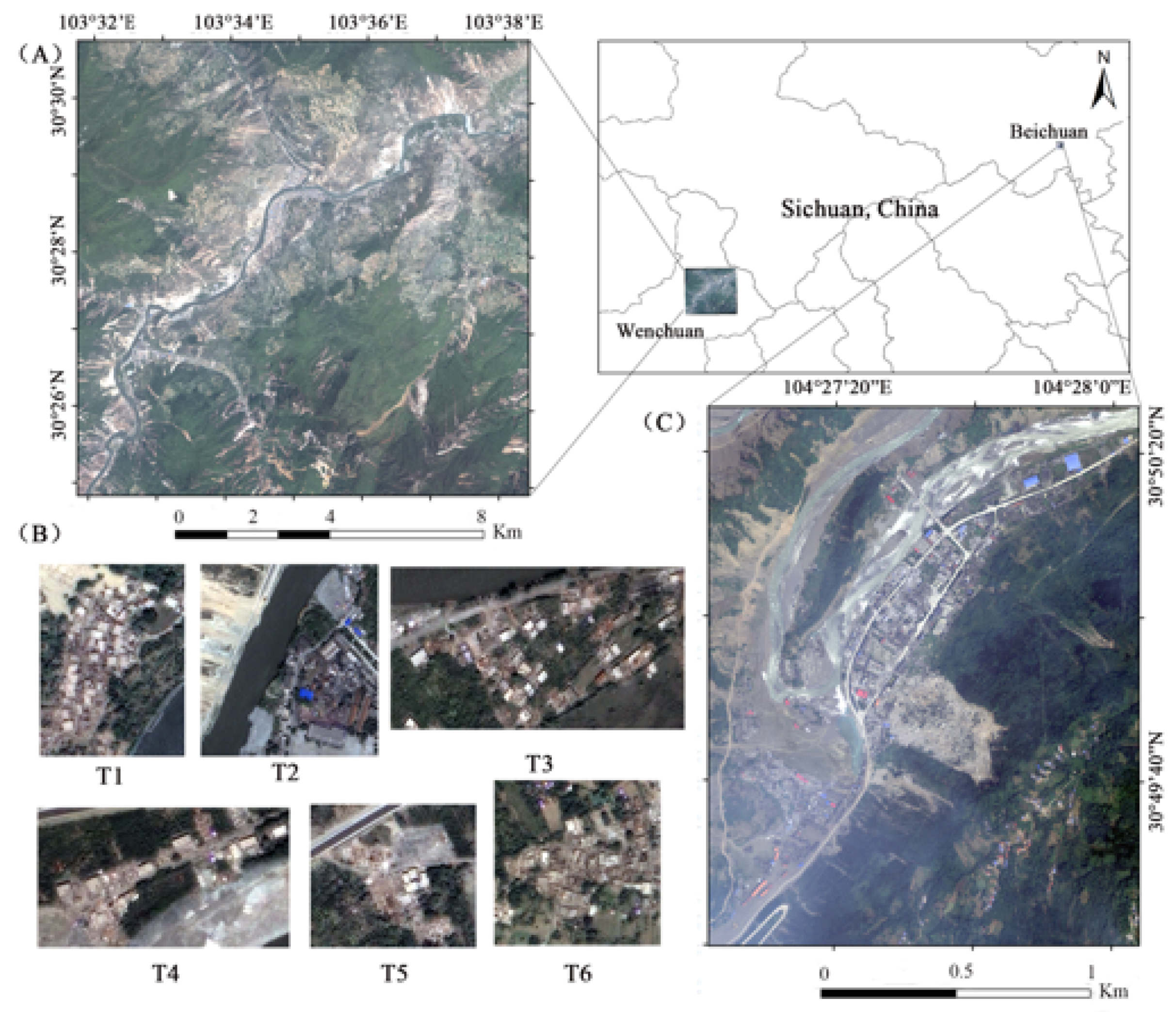
2.2.1. Wenchuan Dataset
The Ikonos satellite images covering part of the Wenchuan area was acquired on 23 May 2008, 11 days after the Earthquake. The image resolution is 1 m after Gram-Schmidt pan-sharpening. Only the RGB bands were used in the study (Figure 1A).
To explore the geographic transferability of the CNN models for the identification of damaged buildings, this study selected six research sub-regions in the Wenchuan area, covering landslide, building collapse, including rural buildings and industrial workshops, which can better cover different post-disaster building patterns (Figure 1B). To get a more reliable ground truth data, the labeling of building damage partly referred to the work in literature [22].
2.2.2. Beichuan Dataset
The image used in Beichuan County was an aerial photo acquired on 13 May 2008, one day after the Earthquake, at a spatial resolution of 0.5 m. Only the aerial photos covering the Zhangcha Town and surrounding area were chosen and processed (Figure 1C).
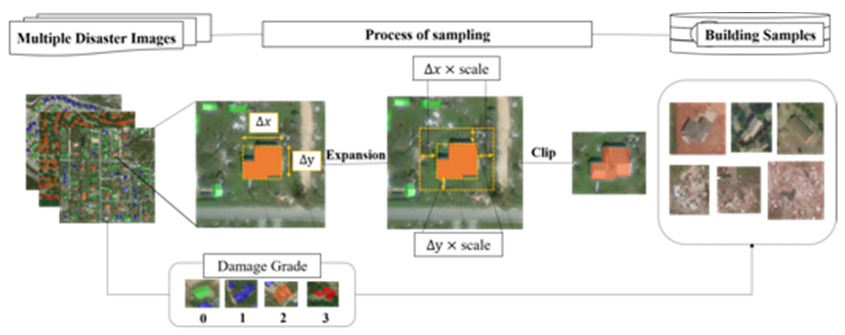
2.3. Sampling
Generating the training samples is an important part of deep learning classification tasks. The quality of the training samples has a direct impact on the learning effect of a network model. Currently, there are several methods to prepare the samples at the building-level [25,26,29]. Such as (1) the whole image was divided into sub-images by using the tile-based image split analysis technique. With the help of the post-earthquake ground survey data, tiles containing buildings were selected as samples [29]; (2) the whole image was clipped by block vector data, then a fixed-size sliding window was used to scan and cut the minimum bounding box of each block to derive sub-images. The samples were then screened by a threshold of their overlapping area with the block unit [25], and (3) the sample set was developed based on a single building, all the samples had a fixed size, pixels outside the building were padding by 0 [26].
In our study, the training samples were prepared based on the single building method. First, the minimum bounding rectangle of the building polygon was obtained, and then the rectangle box was expanded to a certain extent through the expansion coefficient. Finally, the post-disaster building sample was clipped. The detailed description is shown in Figure 2.
Compared with the method of adding 0 to the pixels around the building, this method can take environmental information around the building into account. A dynamic expansion operation according to the size of the building itself can also control the amount of surrounding environment information in a suitable range. At the same time, when a building is seriously damaged or collapsed, the shape of the building changes so much that it extends beyond the polygon. Expanding the boundary can contain the damage pattern more completely. Through the test, the ultimate expansion coefficient was identified to be 0.4. At this scale, there is not too much background interference around the undamaged building samples; in the case of completely collapsed buildings, the sample also covers the whole picture of the damage pattern better.
Table 1 shows the basic information of the samples obtained from the xBD dataset, the Wenchuan and Beichuan images. The intact or slightly-damaged buildings in the Wenchuan and Beichuan area were labeled as one level since it is too hard to distinguish those two types from the post-disaster RS images.
3. Methods
In this section, we firstly present an overview chart of our work (Figure 3). The CNN base models and training methods used in our experiments were illustrated in Section 3.1 and Section 3.2, respectively. Finally, the adjusted CNN models, experiment setting, and accuracy metrics are described in detail in Section 3.3 and Section 3.4.
3.1. CNN Base Models
A significant advantage of the CNN is that it can automatically extract deep level characteristics of the images without the manual feature extraction required in traditional machine learning algorithms. At the same time as model training, the most effective abstract features can be extracted, and then these features can be used for classification [54]. A basic CNN includes convolution layers, pooling layers, and full connection layers (FCL). Through the combination of layers, a variety of network models can be constructed. Four networks, namely VGG16 [59], Inception V3 [60], DenseNet121 [61], and Resnet50 [62] were chosen as the base networks to explore the feature extraction ability of different CNN network structures. These four networks are represented in the structure, and all of them have already been adopted in damaged building identification in some studies [25,48,49,51]. Currently, these four base networks are readily available alongside pre-trained weights for utilization in the Keras library. Figure 3B shows the base unit of each network in the baseline rectangle box.
3.2. Training Method for the Networks
A CNN contains a large number of parameters. Training from scratch to produce a well-performing CNN requires a lot of training data, usually in the order of millions [63]. For a specific task without a large amount of training sample, the use of a pre-trained network is a good solution. The pre-trained network is usually based on large datasets. The spatial hierarchical structure of the features learned by the network can be effectively used as a general model of the visual world to deal with other computer vision problems. There are two ways to use the pre-trained network. One is to use the pre-trained CNN model as a feature extraction tool in which the weight of the convolution basis of the pre-trained network is frozen so that it can only participate in the forward propagation but not in the backward propagation. When the new data are run on it, features are directly extracted and assigned to the new classifier to realize the classification and recognition of the target task. In this paper, this training strategy is termed “CNN-F”. The other way is to fine-tune the pre-trained models [42]. Layers near the top are unfrozen and trained together with the fully connected layers to obtain new model weights for the target task. This training strategy is termed “CNN-T”.
We compared the performance of the two strategies of applying the pre-trained CNNs. The initial weights of the four base networks were the network weights pre-trained on the ImageNet dataset. Previous studies showed that the more layers are fine-tuned, the better the model is [48]. Thus, all layers were set to be trainable in the fine-tune steps.
3.3. The Adjusted CNN Models and Experimental Settings
When using the pre-trained network, the number of neurons in the fully connected layer should be adjusted according to the target task. Moreover, the architecture of the pre-trained network can be adjusted by adding or removing layers to make the network more suitable for the target task [42]. In this study, for each base network, we firstly replaced the last layer of the base network with three fully connected layers. The number of neurons in the last fully connected layer, namely the output layer, is set to 2 or 3 as this study aims at classifying the disaster-damaged buildings into two or three categories. The function of the other two fully connected layers prior to the output layer is to avoid the information loss caused by the sudden decline of dimensions. The dimension of the two added layers were 1024 and 256 respectively. The activation function of these two layers is ReLU, while the activation function in the output layer is determined according to the number of neurons. When the target is two classes, the activation function is Sigmoid, while for 3 classes it is Softmax. The dropout ratio is 0.5. Figure 3B shows the adjusted architecture in detail. The model was built under the Keras 2.3.1 and TensorFlow 2.3.1 framework on NVIDIA GTX 1080ti GPU. Table 2 is a detailed summary of the experiment settings.
In the model training, we used data augmentation to overcome the overfitting problem [64]. The ImageDataGenerator tool under the Keras framework can realize a real-time amplification of the data. In our study, according to the characteristics of the buildings, flip and rotation operations were used for the training samples. In addition, each sample is centralized and normalized. The parameters of the training network were set as follows: the learning rate was set to 0.0001, the batch size was 32, the loss function was cross-entropy. The optimizer was Adam, which combined the advantages of momentum and RMSprop, and made the model quickly and stably descend. To shorten the training time, we used the early stopping strategy. When the accuracy of the validation set does not change significantly, the training process was stopped to save the training time.
3.4. Accuracy Metrics
In the field of deep learning, model evaluation is as important as model training. In our study, overall accuracy, F1 score [65], and Kappa coefficients [66] were selected to measure the performance of the training samples. Overall accuracy is the proportion of correctly classified samples in all predicted samples. Sometimes, the performance of the model cannot be well evaluated by using accuracy alone. When the number of samples is not balanced, the F1 score and Kappa coefficients can better reflect the actual advantages and disadvantages of the model. The F1 score is calculated based on recall and precision. Precision refers to the proportion of “true” samples judged by all systems to be true. Recall refers to the proportion of “true” in all really true samples. The Kappa coefficient tests the consistency between the predicted and the actual results, usually in the range of 0–1. The consistency of the results is above moderate with a Kappa coefficient greater than 0.4. The calculation is based on the confusion matrix. In the confusion matrix, True positive (TP) is the positive sample predicted by the model, True negative (TN) is the negative sample predicted as negative by the model; false positive (FP) is the negative sample predicted as positive by the model, and false-negative (FN) is the negative sample predicted as positive by the model. See Equations (1)–(5) for relevant calculations:
In Equation (5), n is the total number of samples, m is the number of classification categories, is the sum of elements in row i of the corresponding confusion matrix, and is the sum of elements in column i.
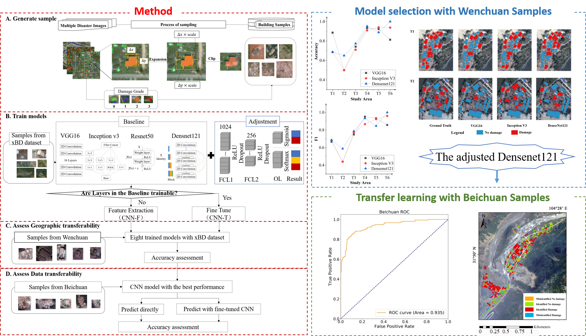
4. Results
In this section, we first explored the performance of four adjusted pre-trained CNNs and two training strategies for identifying disaster-damaged buildings based on the samples obtained from the xBD dataset. Second, the networks with better performance on the xBD dataset were selected and used to explore the geographical transferability of the network using the Wenchuan sample set, namely the prediction ability in locations not seen before. Finally, based on the building samples obtained from the aerial photos in the Beichuan area, we examined the applicability of the network trained with satellite image samples to the identification of damaged buildings from the aerial imagery. Table 3 shows the number of training, validation, and testing samples used in the experiment.
4.1. CNN Performance on the xBD Dataset
A large number of no-damaged samples were generated from xBD, 10 times more than that of the other three types (see Table 1). The imbalance of samples would affect the training of the models. Considering that a greater number of samples leads to a longer training time, we used the down-sampling method to test the performance of the four adjusted CNN models. The specific method was to randomly select 15000 sample images from the no-damage class, which were then integrated with samples in the other three categories to form the training sample set. Among them, 90% of the samples were used for training, 5% for validation, and 5% for testing. The specific number of samples can be found in Table 3.
The four adjusted pre-trained networks were trained by the two training strategies (i.e., CNN-F and CNN-T) based on the xBD sample set. Table 4 shows the prediction results on the xBD test sample set. It can be seen that the pre-trained models trained by CNN-F had a poor performance for disaster-damaged buildings. Among the four adjusted pre-trained networks, the feature representation of the adjusted pre-trained VGG16 model was relatively good for identifying disaster-damaged buildings with a Kappa coefficient of 0.49, while the remaining three pre-trained networks cannot identify disaster-damaged buildings well. Therefore, it is necessary to use post-disaster building samples to fine-tune the weights of the CNN models.
After the fine-tuning process, each network learned the characteristics of disaster-damaged buildings to varying degrees. The performance of each network was also improved accordingly. In addition to the adjusted pre-trained ResNet50, the accuracy of the adjusted pre-trained VGG16, Inception V3, and DenseNet121 are all over 80%; the Kappa coefficient is greater than 0.6 (Table 4). In terms of the testing samples derived from the xBD dataset, the fine-tuned VGG-16 model was slightly better than DenseNet121 and Inception V3.
4.2. Geographic Transferability of the CNN Models
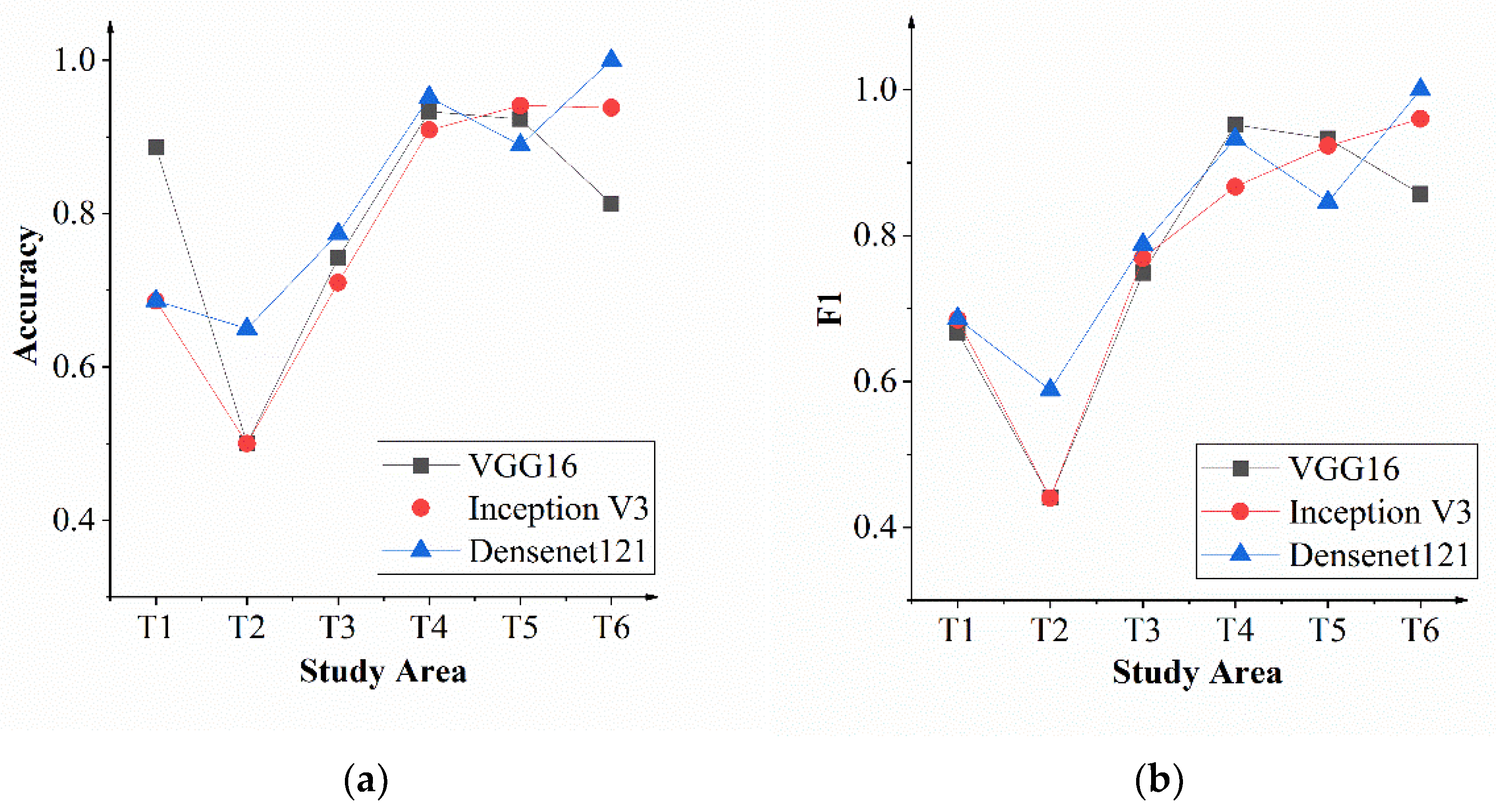
In the eight adjusted pre-trained networks trained with the xBD sample set, the adjusted pre-trained VGG16 (CNN-T), Inception V3 (CNN-T), and DenseNet121 (CNN-T) with better performance were selected to explore their applicability in geographic areas that the models had not seen before. Figure 4 shows the accuracy and F1 score of three CNNs in six sub-study areas of Wenchuan County. The accuracy of the three CNNs in T1 and T2 was relatively low than that on the xBD testing set. The three models achieved much better prediction in T4, T5, and T6. On the whole, the classification performance of the adjusted pre-trained DenseNet121 in the six sub-study areas was relatively stable.
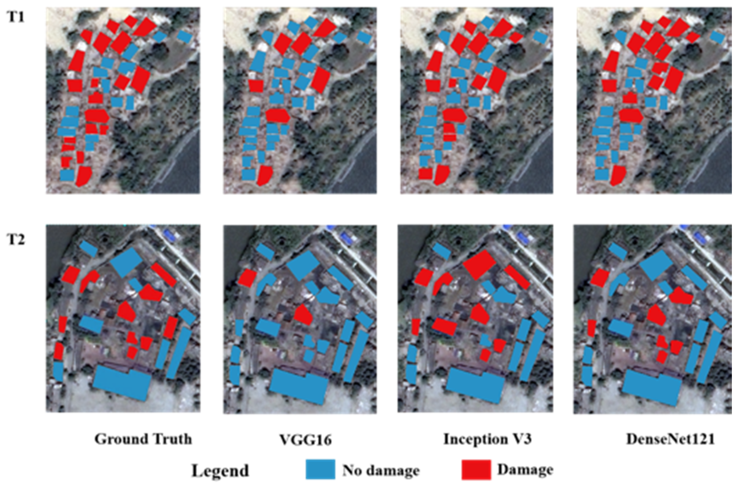
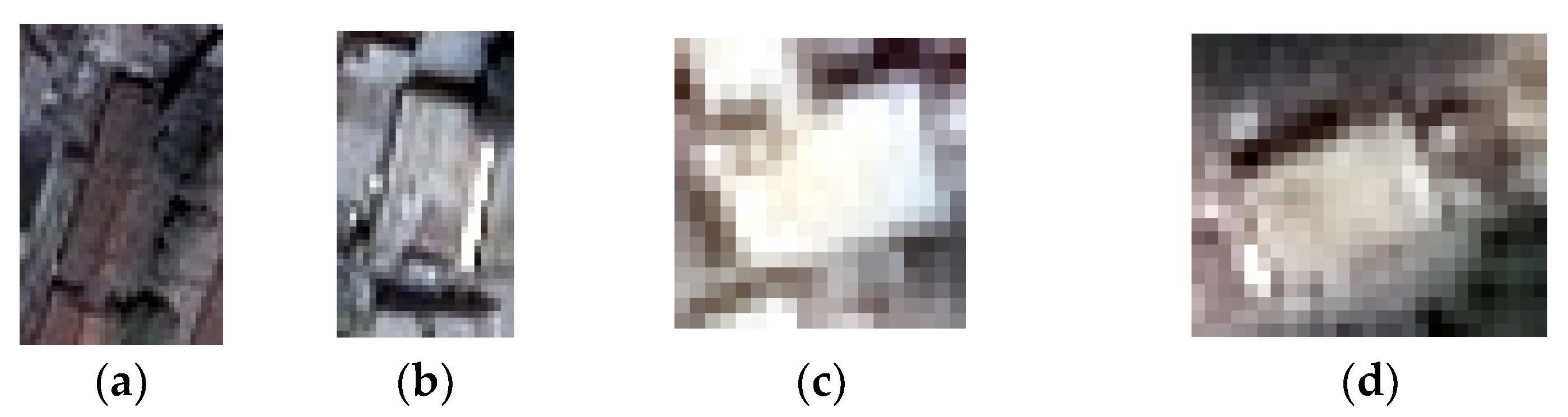
Figure 5 shows the prediction results in the T1 and T2 regions. It can be seen that T1 was a rural area, and the relatively small buildings in this area made it difficult to manually interpret the building damage from post-earthquake satellite images. This would lead to relatively large human errors, which were a very important reason for the low classification accuracy in the T1 region. For the T1 area, comparing the three adjusted CNNs, the performance of VGG16 was poor. After training, Inception V3 and DenseNet121 had better recognition ability for disaster-damaged buildings and could identify most of them correctly. In the T2 area, the structure of buildings showed a different pattern from T1. Compared with other research areas, the buildings in the T2 area were relatively large, where the disaster damage of the building might be effectively evaluated from the remote sensing images. Unfortunately, due to the disordered internal environment and the diversity of the shapes and structures of the buildings, it was also difficult for the networks to correctly distinguish the earthquake-damaged buildings from those complicated but intact buildings. Specifically, VGG16 had poor identification ability which failed in identifying most of the damaged buildings. The recognition abilities of Inception V3 and DensenNet121 were relatively better, but there were missing points of no-damaged buildings. Some damaged buildings, such as Figure 6a,b, were not identified. That might be because the structural damage was not very obvious.
In the T3, T4, T5, and T6 regions, the model had good recognition ability for earthquake-damaged buildings with only a few misclassifications. The qualitative analysis of the misclassification showed that the error in Figure 6c was probably due to the sample making process. When the sample was subset from the image, part of the adjacent building was cut in, which caused the sample to look like a damaged building. Sample in Figure 6d was also misclassified as damaged building. That might result from the complex surrounding environment around the building with lots of debris.
4.3. Applicability of the Models in Aerial Images
The adjusted DenseNet121 that is relatively stable with satellite images was used to examine the transferability of identifying earthquake-damaged buildings from aerial images. The 357 samples obtained from the Beichuan aerial photos were randomly divided into eight sample subsets, named S1–S8. S1–S6 sample subsets were used to fine-tune the network. S7 was used for validation and testing respectively. Table 5 shows the results predicted by the adjusted DenseNet121 model pre-trained with xBD samples and the fine-tuned model with samples from the Beichuan region. The pre-trained model based on the xBD dataset had poor prediction on damaged buildings in the Beichuan area, and consequently, it could not be directly applied to an aerial photo. This indicates that even if the aerial photos have close sub-meter spatial resolution with the satellite data in the xBD dataset, the performance of the model trained with samples from satellite images is not good when the model was applied to the aerial photos. Therefore, it is necessary to use a small number of building samples obtained from the aerial images after the Earthquake to help the pre-trained network with satellite-image samples learn the characteristics from the aerial photo. The performance of the network was much improved after the transfer learning (see Table 5). The recall of the damaged buildings increased from 47.4% to about 80%. However, with the increase in the number of samples, the prediction overall performance of the model remained at a relatively stable level. Compared with the network only fine-tuned with S1, using the S1 and S2 to fine-tune the network improved the recall rate of the no-damage class. Considering the cost of preparing training samples and the accuracy of the model, our experiment shows that using only part of building samples in the prediction area to fine-tune the adjusted DenseNet121 model pre-trained with satellite-image samples could ensure rapid and relatively accurate identification of damaged buildings from the aerial photo.
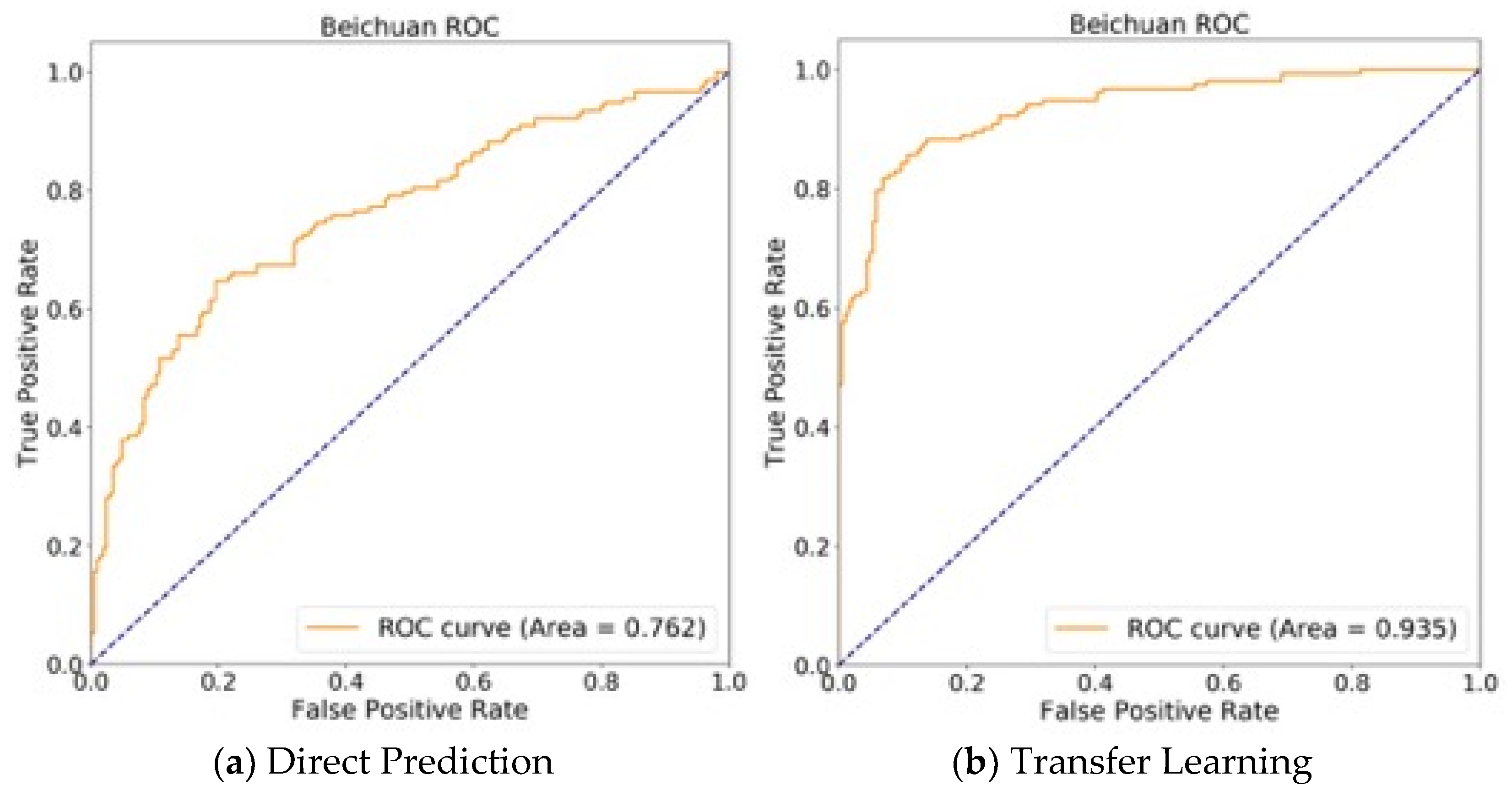
Figure 7 is the receiver operating characteristic (ROC) curve for the classification of all the samples of Beichuan county predicted by the pre-trained adjusted DenseNet121 model directly (see Figure 7a) and by the fine-tuned one with the S1 and S2 (see Figure 7b). It can be seen that the result was improved with the fine-tuning process.
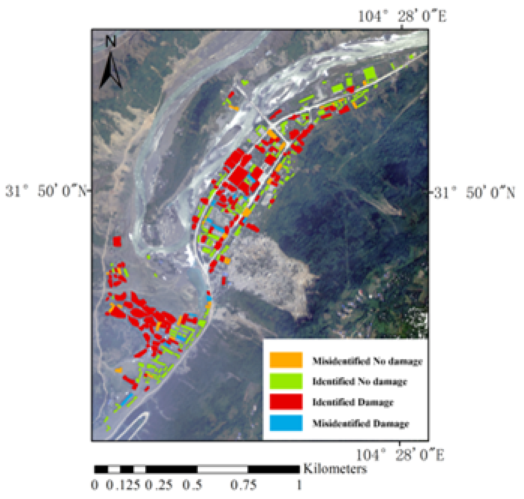
Afterward, the adjusted DenseNet121 model fine-tuned with S1 and S2 sample sets were utilized to produce a classification map of the Beichuan County (Figure 8). A visual check indicates that most of the damaged and undamaged buildings can be identified well. The buildings in red color and green color indicate correct identification of damaged buildings and intact buildings from the aerial photos using our proposedDenseNet121 model, respectively. The buildings in orange color and blue color denote wrong identification of the intact buildings and damaged buildings, respectively.
5. Discussion
Due to the difficulty in preparing sufficient training samples of damaged buildings, it is a pain for using CNN models to rapid retrieve disaster-damaged building information from remote sensing images. In this study, we used samples generated from the public disaster image dataset xBD to train and evaluate the adjusted models based on four typical CNNs, namely VGG-16, Inception v3, DenseNet121, and Resnet50. After that, we also examined the geographic transferability of the adjusted CNN models with better performance in the Wenchuan County. Finally, the adjusted DenseNet with a relatively stable performance was applied in the Beichuan area to figure out its data transferability to aerial photos
The imbalance of training sample distribution is quite common in the preparation of training samples for earthquake disaster. It usually affects the training accuracy of a network model. In addition, to meet the requirement of disaster loss assessment, it is significant but difficult to classify earthquake-affected buildings into a more detailed damage category from post-earthquake satellite or aerial image data. We will address these two problems further in the following section.
5.1. Impact of Sample Imbalance
The building training samples prepared from the xBD dataset imagery dataset contain a large number of intact building samples. The distribution of different types of samples (i.e., no damage, minor damage, major damage and destroyed) is much unbalanced, which could affect the learning process of the networks. As mentioned before, the methods that deal with the imbalance problem can be divided into three categories: data level, algorithm level, and a combination method [26]. The data-level method is mainly resampling, which can be further divided into up-sampling and down-sampling. The up-sampling is to expand the scale of the category with insufficient sample size by using data augmentation and other methods, while down-sampling is to randomly select categories that contain more samples to ensure that the number of samples in each category is balanced. The most commonly used algorithm to solve the imbalance problem is the cost-sensitive method, which assigns different weights to different categories according to their numbers of samples, and applies them to the calculation of model loss function.
We only compared down-sampling and the cost-sensitive method. Data up-sampling is not within the scope of this paper because of the large amount of data involved. Table 6 shows the prediction results of the adjusted DenseNet121 model trained without using the balance method and trained with two balance methods. With the balance method, the performance of the model was improved. Compared to the two balance methods, the cost-sensitive method can enhance the ability to identify disaster-damaged buildings, but it had a significant impact on the identification of no damage class. With higher accuracy, F1 score, and Kappa coefficient in both the xBD test set and samples of Wenchuan, data down-sampling ensured both the accuracy of the two categories and a shorter training time, which is a better choice in our case.
5.2. Detailed Classification of Building Damage Levels
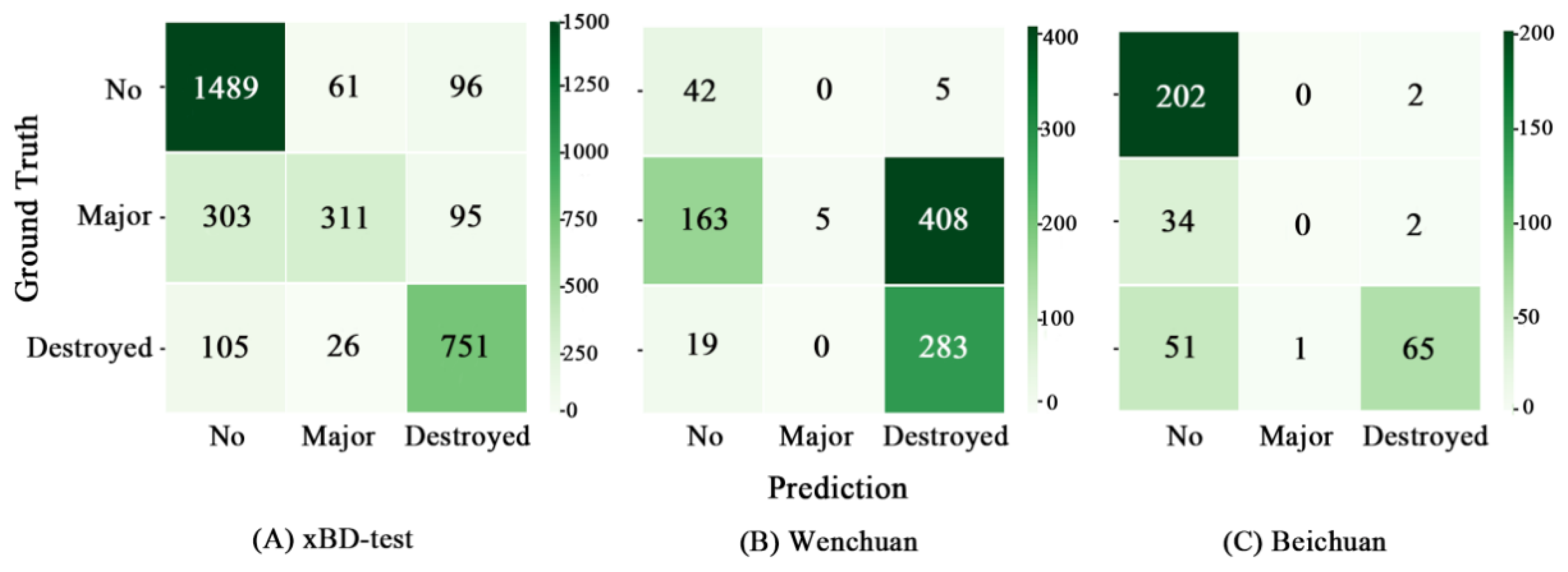
Since four types of building labels in the public dataset xBD were predefined, this study also attempted to explore the possibility of predicting more detailed levels of disaster-damaged damage. Unfortunately, the prediction results of the adjusted DenseNet model were not satisfactory when the model was trained on the three-class labels, i.e., no damage, major damage, and destroyed damage. Figure 9 shows the confusion matrix of the adjusted DenseNet121 model tested on the xBD testing set, Wenchuan and Beichuan dataset. The performance on the xBD testing set was relatively good. Most no-damaged and destroyed buildings were predicted correctly, but the major damaged buildings were not identified properly. Nearly half of the severely damaged buildings were classified as an intact building, and a small part of that were misclassified as the destroyed ones. This situation was more obvious in the research areas that the network had not seen. It can be seen from the confusion matrices that the vast majority of severely damaged buildings in the Wenchuan dataset were misclassified as collapsed buildings, while the buildings with major damage in Beichuan were more likely to be predicted as the no damage type. As a result, the number of buildings with major damage was seriously underestimated in the prediction.
We further analyzed the results to figure out the reason behind the unsatisfactory results. When the disaster-induced building damage was classified into three categories, the main reason for better performance in the xBD testing set was that the geographic locations of the testing samples and the training ones were the same. Consequently, the model learned similar features from them, so it could identify the disaster-damaged buildings in the testing set with higher accuracy. However, for areas that had not been seen by the network, due to the differences in the size, structure, and surrounding environment of buildings, it was difficult to accurately predict more detailed building damage classes because the network had not learned the characteristics of the specific research areas, even with the model trained based on samples from various satellite images. Secondly, the human error of identifying the seriously damaged buildings is unneglectable. Compared with the completely collapsed buildings, the patterns of severely damaged buildings were more complex and diverse, and the differences between them were more subjective. Whether it was the xBD dataset or the testing data of the Wenchuan earthquake, it was difficult to avoid the error in the process of label calibration, which also had a certain impact on the prediction results of the model. For example, severely damaged buildings might be misinterpreted as intact buildings because the damage was difficult to be visually identified from the post-earthquake remote sensing images, and some intact buildings might be misinterpreted as damaged buildings because of their complex structure or special architectural style.
In summary, for the building samples acquired from the xBD dataset, since there were many more intact building samples, it is necessary to deal with the imbalanced learning problem. Our experiment indicated that the random data down-sampling method could reduce down the impact of imbalance learning and guarantee both accuracy and efficiency of the model. The attempt of using the CNN model trained with post-satellite-image samples from xBD to identify more detailed damage levels of disaster-affected buildings with post-disaster data did not yield a satisfactory prediction. We found that it was difficult for the CNN model to correctly identify earthquake-affected buildings that were badly damaged but not collapsed based on satellite remote sensing images. The collapsed or close to collapsed buildings can be well-identified only. Buildings with slight and moderate damage were prone to be confused with intact buildings. Severely damaged buildings might be classified as either intact or collapsed buildings, depending on their damage form and the complexity of the surrounding environment. Some new remote sensors or new remote sensing systems such as Unmanned Aerial Vehicle (UAV) systems might enhance the identification of detailed damage information of buildings in disasters. However, from the perspective of emergency rescue and earthquake casualty estimation, the identification of collapsed buildings can provide data support for casualty estimation.
6. Conclusions
This paper evaluated the performance of the four typical CNN networks in the identification of earthquake-damaged building information from satellite and aerial photos. The public disaster dataset xBD was used to prepare sufficient training samples of building images for training the four adjusted CNN models, namely VGG16, Inception V3, Resnet50, and DenseNet121. The transferability of the CNN models pre-trained with xBD samples was verified with the VHR satellite image samples of the Wenchuan area and aerial photo samples of the Beichuan area acquired right after the 2008 Wenchuan Mw 7.9 earthquake. The adjusted DenseNet121 pre-trained with the xBD samples performed best among four chosen CNN models. The down-sampling method can be used to reduce the impact of the imbalance problem between the classes “no damage” and “damaged” samples on the model training process, and achieve better identification of collapsed buildings without compromising the prediction accuracy of the class “no damage”. When the adjusted DenseNet121 model pre-trained with the VHR satellite image samples generated from the xBD dataset was directly used in the identification of damaged buildings from the aerial photo data of the Beichuan area, it performed quite poor and had low transferability between different sensor data (e.g., satellite versus aerial). However, our experiment indicated that with the fine-tuning process, the performance of the adjusted DenseNet121 pre-trained on satellite-image samples can be improved with a small portion of building samples from the aerial photos of Beichuan. The overall accuracy of the model without and with fine-tuning was improved from 64.3% to 88.9% and the recall rate for the class “damaged” building was ameliorated from 47.4% to 89.5%. The improved DenseNet121 model pre-trained with large xBD samples can meet the requirement for rapid understanding of the locations of collapsed buildings in an earthquake disaster and provide important support for emergency rescue.
We also found that a more detailed classification of earthquake-induced buildings damage level (i.e., minor damage, major damage and destroyed) was not satisfactory with the CNN models in the Wenchuan and Beichuan areas, where the 2008 Wenchuan Earthquake took place on 12 May 2008. A certain proportion of major damaged buildings were wrongly classified as intact or collapsed buildings. Future work may explore the usefulness of some new remote sensors such as LiDAR and new remote sensing platforms such as unmanned aerial vehicle systems in the identification of detailed damage levels of buildings caused by disasters such as earthquakes.
Author Contributions
Conceptualization, implementation and draft preparation, W.Y., funding acquisition, conceptualization, and review and editing, X.Z., and data curation, P.L. All authors have read and agreed to the published version of the manuscript.
Funding
This research and APC were funded by the National Key Research and Development Program of Ministry of Science and Technology, China, grant number, 2017YFC1500902, and by the Xinjiang Production and Construction Corps, China, grant number, 2017DB005.
Acknowledgments
We would like to give our thanks to the three reviewers for their constructive comments on our work. We also appreciate the creators of the xBD dataset for producing this valuable public data.
Conflicts of Interest
The authors declare no conflict of interest.
Abbreviations
The following abbreviations are used in this manuscript:
| VHR | Very-High Resolution |
| SAR | Synthetic Aperture Radar |
| OBIA | Object-Based Image Analysis |
| CNN | Convolutional Neural Network |
| RF | Random Forest |
| SVM | Support Vector Machine |
| DL | Deep learning |
| Mw | Moment magnitude |
| RGB | Red, green, blue |
| FEMA | Federal Emergency Management Agency |
| FCL | Full Connection Layer |
| OL | Output layer |
| TP | True positive |
| TN | True negative |
| FP | False positive |
| FN | False negative |
| ReLU | Rectified linear unit |
| AUC | Area under curve |
| F1 | Harmonic mean of precision and recall |
| HPC | High-Performance Computing |
| ROC | Receiver operating characteristic curve |
| UAV | Unmanned Aerial Vehicle |
References
- Jaiswal, K.; Wald, D.J. Creating a Global Building Inventory for Earthquake Loss Assessment and Risk Management; US Geological Survey: Denver, CO, USA, 2008.
- Murakami, H. A simulation model to estimate human loss for occupants of collapsed buildings in an earthquake. In Proceedings of the Tenth World Conference on Earthquake Engineering, Madrid, Spain, 19–24 July 1992; pp. 5969–5976. [Google Scholar]
- Coburn, A.W.; Spence, R.J.; Pomonis, A. Factors determining human casualty levels in earthquakes: Mortality prediction in building collapse. In Proceedings of the Tenth World Conference on Earthquake Engineering, Madrid, Spain, 19–24 July 1992; pp. 5989–5994. [Google Scholar]
- Brunner, D.; Lemoine, G.; Bruzzone, L. Earthquake damage assessment of buildings using VHR optical and SAR imagery. IEEE Trans. Geosci. Remote Sens. 2010, 48, 2403–2420. [Google Scholar] [CrossRef] [Green Version]
- Huyck, C.K.; Adams, B.J.; Cho, S.; Chung, H.-C.; Eguchi, R.T. Towards rapid citywide damage mapping using neighborhood edge dissimilarities in very high-resolution optical satellite imagery—Application to the 2003 Bam, Iran, earthquake. Earthq. Spectra 2005, 21, 255–266. [Google Scholar] [CrossRef]
- Janalipour, M.; Mohammadzadeh, A. Building damage detection using object-based image analysis and ANFIS from high-resolution image (Case study: BAM earthquake, Iran). IEEE J. Sel. Top. Appl. Earth Obs. Remote Sens. 2015, 9, 1937–1945. [Google Scholar] [CrossRef]
- Yamazaki, F.; Liu, W. Remote sensing technologies for post-earthquake damage assessment: A case study on the 2016 Kumamoto earthquake. In Proceedings of the Keynote Lecture, 6th Asia Conference on Earthquake Engineering, Cebu City, Philippines, 22–24 September 2016. [Google Scholar]
- Pesaresi, M.; Gerhardinger, A.; Haag, F. Rapid damage assessment of built-up structures using VHR satellite data in tsunami-affected areas. Int. J. Remote Sens. 2007, 28, 3013–3036. [Google Scholar] [CrossRef]
- Ehrlich, D.; Guo, H.; Molch, K.; Ma, J.; Pesaresi, M. Identifying damage caused by the 2008 Wenchuan earthquake from VHR remote sensing data. Int. J. Digit. Earth 2009, 2, 309–326. [Google Scholar] [CrossRef]
- Li, L.; Liu, X.; Chen, Q.; Yang, S. Building damage assessment from PolSAR data using texture parameters of statistical model. Comput. Geosci. 2018, 113, 115–126. [Google Scholar] [CrossRef]
- Chen, Q.; Nie, Y.; Li, L.; Liu, X. Buildings damage assessment using texture features of polarization decomposition components. J. Remote Sens. 2017, 21, 955–965. [Google Scholar]
- Gong, L.; Wang, C.; Wu, F.; Zhang, J.; Zhang, H.; Li, Q. Earthquake-induced building damage detection with post-event sub-meter VHR TerraSAR-X staring spotlight imagery. Remote Sens. 2016, 8, 887. [Google Scholar] [CrossRef] [Green Version]
- Bai, Y.; Adriano, B.; Mas, E.; Koshimura, S. Machine Learning Based Building Damage Mapping from the ALOS-2/PALSAR-2 SAR Imagery: Case Study of 2016 Kumamoto Earthquake. J. Disaster Res. 2017, 12, 646–655. [Google Scholar] [CrossRef]
- Dou, A.; Ma, Z.; Huang, W.; Wang, X.; Yuan, X. Automatic identification approach of building damages caused by earthquake based on airborne LiDAR and multispectral imagery. Remote Sens. Inf. 2013, 28, 103–109. [Google Scholar]
- Wang, X.; Li, P. Extraction of urban building damage using spectral, height and corner information from VHR satellite images and airborne LiDAR data. ISPRS J. Photogramm. Remote Sens. 2020, 159, 322–336. [Google Scholar] [CrossRef]
- Li, M.; Cheng, L.; Gong, J.; Liu, Y.; Chen, Z.; Li, F.; Chen, G.; Chen, D.; Song, X. Post-earthquake assessment of building damage degree using LiDAR data and imagery. Sci. China Ser. E Technol. Sci. 2008, 51, 133–143. [Google Scholar] [CrossRef]
- Sun, J.; Chen, L.; Xie, Y.; Zhang, S.; Jiang, Q.; Zhou, X.; Bao, H. Disp R-CNN: Stereo 3D Object Detection via Shape Prior Guided Instance Disparity Estimation. In Proceedings of the IEEE/CVF Conference on Computer Vision and Pattern Recognition, Seattle, WA, USA, 13–19 June 2020; pp. 10548–10557. [Google Scholar]
- Franceschetti, G.; Guida, R.; Iodice, A.; Riccio, D.; Ruello, G.; Stilla, U. Building feature extraction via a deterministic approach: Application to real high resolution SAR images. In Proceedings of the 2007 IEEE International Geoscience and Remote Sensing Symposium, Barcelona, Spain, 13–27 July 2007; pp. 2681–2684. [Google Scholar]
- Xue, T.; Zhang, J.; Li, Q. Extraction of earthquake damage buildings from multi-source remote sensing data based on correlation change detection and object-oriented classification techniques. Acta Seismol. Sin. 2016, 38, 496–505. [Google Scholar]
- Tong, X.; Hong, Z.; Liu, S.; Zhang, X.; Xie, H.; Li, Z.; Yang, S.; Wang, W.; Bao, F. Building-damage detection using pre-and post-seismic high-resolution satellite stereo imagery: A case study of the May 2008 Wenchuan earthquake. ISPRS J. Photogramm. Remote Sens. 2012, 68, 13–27. [Google Scholar] [CrossRef]
- Tiede, D.; Lang, S.; Füreder, P.; Hölbling, D.; Hoffmann, C.; Zeil, P. Automated damage indication for rapid geospatial reporting. Photogramm. Eng. Remote Sens. 2011, 77, 933–942. [Google Scholar] [CrossRef]
- Song, D.; Tan, X.; Wang, B.; Zhang, L.; Shan, X.; Cui, J. Integration of super-pixel segmentation and deep-learning methods for evaluating earthquake-damaged buildings using single-phase remote sensing imagery. Int. J. Remote Sens. 2020, 41, 1040–1066. [Google Scholar] [CrossRef]
- Ma, H.; Liu, Y.; Ren, Y.; Yu, J. Detection of Collapsed Buildings in Post-Earthquake Remote Sensing Images Based on the Improved YOLOv3. Remote Sens. 2020, 12, 44. [Google Scholar] [CrossRef] [Green Version]
- Salehi, B.; Ming Zhong, Y.; Dey, V. A review of the effectiveness of spatial information used in urban land cover classification of VHR imagery. Int. J. Geoinform. 2012, 8, 35. [Google Scholar]
- Ma, H.; Liu, Y.; Ren, Y.; Wang, D.; Yu, L.; Yu, J. Improved CNN Classification Method for Groups of Buildings Damaged by Earthquake, Based on High Resolution Remote Sensing Images. Remote Sens. 2020, 12, 260. [Google Scholar] [CrossRef] [Green Version]
- Ji, M.; Liu, L.; Buchroithner, M. Identifying Collapsed Buildings Using Post-Earthquake Satellite Imagery and Convolutional Neural Networks: A Case Study of the 2010 Haiti Earthquake. Remote Sens. 2018, 10, 1689. [Google Scholar] [CrossRef] [Green Version]
- Miura, H.; Aridome, T.; Matsuoka, M. Deep Learning-Based Identification of Collapsed, Non-Collapsed and Blue Tarp-Covered Buildings from Post-Disaster Aerial Images. Remote Sens. 2020, 12, 1924. [Google Scholar] [CrossRef]
- Chen, M.; Wang, X.; Dou, A.; Wu, X. The extraction of post-earthquake building damage information based on convolutional neural network. Int. Arch. Photogramm. Remote Sens. Spat. Inf. Sci. 2018, 42, 161–165. [Google Scholar] [CrossRef] [Green Version]
- Bai, Y.; Gao, C.; Singh, S.; Koch, M.; Adriano, B.; Mas, E.; Koshimura, S. A framework of rapid regional tsunami damage recognition from post-event TerraSAR-X imagery using deep neural networks. IEEE Geosci. Remote Sens. Lett. 2017, 15, 43–47. [Google Scholar] [CrossRef] [Green Version]
- Sui, H.; Liu, C.; Huang, L.; Hua, L. Application of remote sensing technology in earthquake-induced building damage detection. Geomat. Inf. Sci. Wuhan Univ. 2019, 044, 1008–1019. [Google Scholar]
- Wang, H.; Li, Y. Object-oriented damage building extraction. Remote Sens. Inf. 2011, 8, 81–85. [Google Scholar]
- Adriano, B.; Xia, J.; Baier, G.; Yokoya, N.; Koshimura, S. Multi-Source Data Fusion Based on Ensemble Learning for Rapid Building Damage Mapping during the 2018 Sulawesi Earthquake and Tsunami in Palu, Indonesia. Remote Sens. 2019, 11, 886. [Google Scholar] [CrossRef] [Green Version]
- Cooner, A.; Shao, Y.; Campbell, J. Detection of Urban Damage Using Remote Sensing and Machine Learning Algorithms: Revisiting the 2010 Haiti Earthquake. Remote Sens. 2016, 8, 868. [Google Scholar] [CrossRef] [Green Version]
- Janalipour, M.; Mohammadzadeh, A. A Fuzzy-GA Based Decision Making System for Detecting Damaged Buildings from High-Spatial Resolution Optical Images. Remote Sens. 2017, 9, 349. [Google Scholar] [CrossRef] [Green Version]
- Wieland, M.; Liu, W.; Yamazaki, F. Learning Change from Synthetic Aperture Radar Images: Performance Evaluation of a Support Vector Machine to Detect Earthquake and Tsunami-Induced Changes. Remote Sens. 2016, 8, 792. [Google Scholar] [CrossRef] [Green Version]
- Breiman, L. Random forests. Mach. Learn. 2001, 45, 5–32. [Google Scholar] [CrossRef] [Green Version]
- Cortes, C.; Vapnik, V. Support-vector networks. Mach. Learn. 1995, 20, 273–297. [Google Scholar] [CrossRef]
- Harirchian, E.; Lahmer, T.; Kumari, V.; Jadhav, K. Application of Support Vector Machine Modeling for the Rapid Seismic Hazard Safety Evaluation of Existing Buildings. Energies 2020, 13, 3340. [Google Scholar] [CrossRef]
- Harirchian, E.; Kumari, V.; Jadhav, K.; Raj Das, R.; Rasulzade, S.; Lahmer, T. A Machine Learning Framework for Assessing Seismic Hazard Safety of Reinforced Concrete Buildings. Appl. Sci. 2020, 10, 7153. [Google Scholar] [CrossRef]
- Roeslin, S.; Ma, Q.; Juárez-Garcia, H.; Gómez-Bernal, A.; Wicker, J.; Wotherspoon, L. A machine learning damage prediction model for the 2017 Puebla-Morelos, Mexico, earthquake. Earthq. Spectra 2020, 36, 314–339. [Google Scholar] [CrossRef]
- Harirchian, E.; Lahmer, T. Developing a hierarchical type-2 fuzzy logic model to improve rapid evaluation of earthquake hazard safety of existing buildings. Structures 2020, 28, 1384–1399. [Google Scholar] [CrossRef]
- Vetrivel, A.; Gerke, M.; Kerle, N.; Nex, F.; Vosselman, G. Disaster damage detection through synergistic use of deep learning and 3D point cloud features derived from very high resolution oblique aerial images, and multiple-kernel-learning. ISPRS J. Photogramm. Remote Sens. 2018, 140, 45–59. [Google Scholar] [CrossRef]
- Bhuiyan, M.A.E.; Witharana, C.; Liljedahl, A.K. Use of Very High Spatial Resolution Commercial Satellite Imagery and Deep Learning to Automatically Map Ice-Wedge Polygons across Tundra Vegetation Types. J. Imaging 2020, 6, 137. [Google Scholar] [CrossRef]
- Xu, Z.; Zhang, W.; Zhang, T.; Li, J. HRCNet: High-Resolution Context Extraction Network for Semantic Segmentation of Remote Sensing Images. Remote Sens. 2020, 13, 71. [Google Scholar] [CrossRef]
- Zhang, S.; Li, C.; Qiu, S.; Gao, C.; Zhang, F.; Du, Z.; Liu, R. EMMCNN: An ETPS-Based Multi-Scale and Multi-Feature Method Using CNN for High Spatial Resolution Image Land-Cover Classification. Remote Sens. 2019, 12, 66. [Google Scholar] [CrossRef] [Green Version]
- Bai, Y.; Hu, J.; Su, J.; Liu, X.; Liu, H.; He, X.; Meng, S.; Mas, E.; Koshimura, S. Pyramid Pooling Module-Based Semi-Siamese Network: A Benchmark Model for Assessing Building Damage from xBD Satellite Imagery Datasets. Remote Sens. 2020, 12, 4055. [Google Scholar] [CrossRef]
- Ji, M.; Liu, L.; Du, R.; Buchroithner, M.F. A comparative study of texture and convolutional neural network features for detecting collapsed buildings after earthquakes using pre-and post-event satellite imagery. Remote Sens. 2019, 11, 1202. [Google Scholar] [CrossRef] [Green Version]
- Ji, M.; Liu, L.; Zhang, R.; Buchroithner, M.F. Discrimination of Earthquake-Induced Building Destruction from Space Using a Pretrained CNN Model. Appl. Ences 2020, 10, 602. [Google Scholar] [CrossRef] [Green Version]
- Wheeler, B.J.; Karimi, H.A. Deep Learning-Enabled Semantic Inference of Individual Building Damage Magnitude from Satellite Images. Algorithms 2020, 13, 195. [Google Scholar] [CrossRef]
- Amirkolaee, H.A.; Arefi, H. CNN-based estimation of pre- and post-earthquake height models from single optical images for identification of collapsed buildings. Remote Sens. Lett. 2019, 10, 679–688. [Google Scholar] [CrossRef]
- Nex, F.; Duarte, D.; Tonolo, F.G.; Kerle, N. Structural building damage detection with deep learning: Assessment of a state-of-the-art cnn in operational conditions. Remote Sens. 2019, 11, 2765. [Google Scholar] [CrossRef] [Green Version]
- Valentijn, T.; Margutti, J.; van den Homberg, M.; Laaksonen, J. Multi-hazard and spatial transferability of a cnn for automated building damage assessment. Remote Sens. 2020, 12, 2839. [Google Scholar] [CrossRef]
- Su, J.; Bai, Y.; Wang, X.; Lu, D.; Zhao, B.; Yang, H.; Mas, E.; Koshimura, S. Technical Solution Discussion for Key Challenges of Operational Convolutional Neural Network-Based Building-Damage Assessment from Satellite Imagery: Perspective from Benchmark xBD Dataset. Remote Sens. 2020, 12, 3808. [Google Scholar] [CrossRef]
- Chen, Y.; Jiang, H.; Li, C.; Jia, X.; Ghamisi, P. Deep feature extraction and classification of hyperspectral images based on convolutional neural networks. IEEE Trans. Geosci. Remote Sens. 2016, 54, 6232–6251. [Google Scholar] [CrossRef] [Green Version]
- Li, Y.; Hu, W.; Dong, H.; Zhang, X. Building damage detection from post-event aerial imagery using single shot multibox detector. Appl. Sci. 2019, 9, 1128. [Google Scholar] [CrossRef] [Green Version]
- Benson, V.; Ecker, A. Assessing out-of-domain generalization for robust building damage detection. arXiv 2020, arXiv:2011.10328. [Google Scholar]
- Gupta, R.; Hosfelt, R.; Sajeev, S.; Patel, N.; Goodman, B.; Doshi, J.; Heim, E.; Choset, H.; Gaston, M. xBD: A Dataset for Assessing Building Damage from Satellite Imagery. arXiv 2019, arXiv:1911.09296. [Google Scholar]
- Fan, X.; Juang, C.H.; Wasowski, J.; Huang, R.; Xu, Q.; Scaringi, G.; van Westen, C.J.; Havenith, H.-B. What we have learned from the 2008 Wenchuan Earthquake and its aftermath: A decade of research and challenges. Eng. Geol. 2018, 241, 25–32. [Google Scholar] [CrossRef]
- Simonyan, K.; Zisserman, A. Very deep convolutional networks for large-scale image recognition. arXiv 2014, arXiv:1409.1556. [Google Scholar]
- Szegedy, C.; Vanhoucke, V.; Ioffe, S.; Shlens, J.; Wojna, Z. Rethinking the inception architecture for computer vision. In Proceedings of the IEEE Conference on Computer Vision and Pattern Recognition, Las Vegas, NV, USA, 27–30 June 2016; pp. 2818–2826. [Google Scholar]
- Iandola, F.; Moskewicz, M.; Karayev, S.; Girshick, R.; Darrell, T.; Keutzer, K. Densenet: Implementing efficient convnet descriptor pyramids. arXiv 2014, arXiv:1404.1869. [Google Scholar]
- He, K.; Zhang, X.; Ren, S.; Sun, J. Deep residual learning for image recognition. In Proceedings of the IEEE Conference on Computer Vision and Pattern Recognition, Las Vegas, NV, USA, 27–30 June 2016; pp. 770–778. [Google Scholar]
- Tajbakhsh, N.; Shin, J.Y.; Gurudu, S.R.; Hurst, R.T.; Kendall, C.B.; Gotway, M.B.; Liang, J. Convolutional neural networks for medical image analysis: Full training or fine tuning? IEEE Trans. Med Imaging 2016, 35, 1299–1312. [Google Scholar] [CrossRef] [PubMed] [Green Version]
- Perez, L.; Wang, J. The effectiveness of data augmentation in image classification using deep learning. arXiv 2017, arXiv:1712.04621. [Google Scholar]
- Chinchor, N.; Sundheim, B.M. MUC-5 evaluation metrics. In Proceedings of the Fifth Message Understanding Conference (MUC-5), Baltimore, MD, USA, 25–27 August 1993. [Google Scholar]
- McHugh, M.L. Interrater reliability: The kappa statistic. Biochem. Med. 2012, 22, 276–282. [Google Scholar] [CrossRef]
Figure 1.
Location of the study area and the remote sensing images after the 2008 Mw7.9 Wenchuan Earthquake: (A) the composite image of the Northeast of Wenchuan County; (B) images for T1–T6 sub-study areas in the Wenchuan County; (C) the image of the Beichuan County.
Figure 1.
Location of the study area and the remote sensing images after the 2008 Mw7.9 Wenchuan Earthquake: (A) the composite image of the Northeast of Wenchuan County; (B) images for T1–T6 sub-study areas in the Wenchuan County; (C) the image of the Beichuan County.

Figure 2.
Workflow for preparing the building samples from the dataset of this study.

Figure 3.
Flowchart of the work, including four steps: (A) to generate samples from the image datasets described in Section 2; (B) to train the CNN models with the samples generated in Step A; (C) to assess geographic transferability with the samples of Wenchuan, and (D) to assess data transferability with the samples of Beichuan.

Figure 4.
Results evaluated by (a) Accuracy and (b) F1 score of the adjusted pre-trained VGG16 (CNN-T), Inception V3 (CNN-T), and DenseNet121 (CNN-T) in the six sub-study areas T1–T6 of Wenchuan County.
Figure 4.
Results evaluated by (a) Accuracy and (b) F1 score of the adjusted pre-trained VGG16 (CNN-T), Inception V3 (CNN-T), and DenseNet121 (CNN-T) in the six sub-study areas T1–T6 of Wenchuan County.

Figure 5.
Comparison of the predicted results of three adjusted CNN models in the T1 and T2 sub-study regions.
Figure 5.
Comparison of the predicted results of three adjusted CNN models in the T1 and T2 sub-study regions.

Figure 6.
Examples of building misclassification in the Wenchuan area. (a,b) are damaged buildings but wrongly classified as no damage in T2; (c) the building with no damage but was wrongly classified as damaged in T4; (d) the building with no damage but wrongly was classified as damaged in T5.
Figure 6.
Examples of building misclassification in the Wenchuan area. (a,b) are damaged buildings but wrongly classified as no damage in T2; (c) the building with no damage but was wrongly classified as damaged in T4; (d) the building with no damage but wrongly was classified as damaged in T5.

Figure 7.
ROC curve for the classification result of all the building samples of Beichuan. (a) prediction from the pre-trained model without fine-tuning process; (b) prediction from the pre-trained model fine-tuned with S1 and S2 samples.
Figure 7.
ROC curve for the classification result of all the building samples of Beichuan. (a) prediction from the pre-trained model without fine-tuning process; (b) prediction from the pre-trained model fine-tuned with S1 and S2 samples.

Figure 8.
Predicted results of earthquake-damaged buildings in Beichuan using the adjusted DenseNet121 model with the fine-tuning process.
Figure 8.
Predicted results of earthquake-damaged buildings in Beichuan using the adjusted DenseNet121 model with the fine-tuning process.

Figure 9.
Confusion matrices of the adjusted DenseNet121 model tested on (A) the xBD-test dataset, (B) the Wenchuan dataset, and (C) the Beichuan dataset.
Figure 9.
Confusion matrices of the adjusted DenseNet121 model tested on (A) the xBD-test dataset, (B) the Wenchuan dataset, and (C) the Beichuan dataset.


Table 1.
Number of samples in various damage levels.
| Dataset | Number of Samples | |||||
|---|---|---|---|---|---|---|
| No. 1 | Minor. 2 | Major. 3 | Destroyed | Total | ||
| xBD | 165,844 | 17,929 | 14,173 | 17,634 | 215,580 | |
| Wenchuan | T1 | 15 | 15 | 5 | 35 | |
| T2 | 9 | 8 | 3 | 20 | ||
| T3 | 11 | 10 | 10 | 31 | ||
| T4 | 4 | 1 | 10 | 15 | ||
| T5 | 5 | 3 | 5 | 13 | ||
| T6 | 3 | 5 | 8 | 16 | ||
| Beyond T1–T6 | - | 261 | 534 | 795 | ||
| Beichuan | 204 | 36 | 117 | 357 | ||
1 No Damage; 2 Minor Damage; 3 Major Damage. The samples for No damage and Minor damage are merged in Wenchuan and Beichuan.
Table 2.
Settings of the CNN Networks in the Experiment.
| HPC Resource | NVIDIA GTX 1080ti GPU |
| DL Framework | Keras 2.3.1, Tensorflow 2.3.1 |
| Compiler | Jupyter Notebook 6.0.3 |
| Program | Python 3.7.0 |
| Optimizer | Adam |
| Loss Function | Cross-entropy |
| Learning rate | 0.0001 |
| Batch size | 32 |
Table 3.
Summary for the corresponding numbers of training, validation, and testing samples used in the experiment.
Table 3.
Summary for the corresponding numbers of training, validation, and testing samples used in the experiment.
| Dataset | Number of Samples | ||||||
|---|---|---|---|---|---|---|---|
| Training | Validation | Testing | |||||
| No | Damage | No | Damage | No | Damage | ||
| xBD | 29,636 | 28,626 | 1647 | 1590 | 1646 | 1591 | |
| Wenchuan | T1 | - | 15 | 20 | |||
| T2 | 9 | 11 | |||||
| T3 | 11 | 20 | |||||
| T4 | 4 | 11 | |||||
| T5 | 5 | 8 | |||||
| T6 | 3 | 13 | |||||
| Beyond T1–T6 | - | - | 795 | ||||
| Beichuan | - | - | - | 25 | 19 | 26 | 19 |
| S1 | 25 | 19 | 25 | 19 | 26 | 19 | |
| S1,2 | 51 | 38 | 25 | 19 | 26 | 19 | |
| S1,2,3 | 76 | 57 | 25 | 19 | 26 | 19 | |
| S1,2,3,4 | 102 | 76 | 25 | 19 | 26 | 19 | |
| S1,2,3,4,5 | 127 | 96 | 25 | 19 | 26 | 19 | |
| S1,2,3,4,5,6 1 | 153 | 115 | 25 | 19 | 26 | 19 | |
Note: 1 S1–S6 in the table is the sample subsets of the Beichuan samples used for transfer learning. See 4.3 for more details.
Table 4.
Accuracy assessment of the predicted results of the four adjusted pre-trained CNN models on the xBD testing dataset using the metrics Accuracy (%), F1, Recall (%), Precision (%), and Kappa.
Table 4.
Accuracy assessment of the predicted results of the four adjusted pre-trained CNN models on the xBD testing dataset using the metrics Accuracy (%), F1, Recall (%), Precision (%), and Kappa.
| Network | Type | Acc. 1 (%) | F1 | Recall | Precision | Kappa | ||
|---|---|---|---|---|---|---|---|---|
| No. 2 | Damage | No. 2 | Damage | |||||
| VGG-16 | CNN-F | 74.7 | 0.746 | 73.8 | 75.6 | 75.8 | 73.6 | 0.49 |
| CNN-T | 83.6 | 0.825 | 88.3 | 78.6 | 81.0 | 86.7 | 0.67 | |
| Inception V3 | CNN-F | 62.0 | 0.622 | 60.4 | 63.7 | 63.2 | 60.8 | 0.24 |
| CNN-T | 80.3 | 0.789 | 85.2 | 75.1 | 78.0 | 83.1 | 0.60 | |
| ResNet50 | CNN-F | 54.8 | 0.530 | 35.2 | 75.1 | 59.4 | 52.8 | 0.1 |
| CNN-T | 63.5 | 0.523 | 95.0 | 37.3 | 61.0 | 87.0 | 0.33 | |
| DenseNet121 | CNN-F | 68.2 | 0.712 | 56.8 | 80.0 | 74.6 | 64.2 | 0.37 |
| CNN-T | 82.1 | 0.805 | 78.7 | 75.1 | 88.9 | 86.8 | 0.64 | |
Note: 1 Accuracy; 2 No Damage.
Table 5.
Accuracy assessment of the prediction results of the adjusted DenseNet121 pre-trained by satellite-image samples fine-tuned with the samples generated from the aerial image of Beichuan using the metrics Accuracy (%), F1, Recall (%), and Kappa.
Table 5.
Accuracy assessment of the prediction results of the adjusted DenseNet121 pre-trained by satellite-image samples fine-tuned with the samples generated from the aerial image of Beichuan using the metrics Accuracy (%), F1, Recall (%), and Kappa.
| Network | Fine-Tune Sample | Test Accuracy (%) | Test F1 Score | Recall | Kappa | |
|---|---|---|---|---|---|---|
| No Damage (%) | Damage (%) | |||||
| DenseNet121 | - | 64.3 | 0.778 | 100 | 47.4 | 0.51 |
| S1 | 82.2 | 0.8 | 80.8 | 84.2 | 0.64 | |
| S1,2 | 86.5 | 0.889 | 92.3 | 84.2 | 0.77 | |
| S1,2,3 | 82.1 | 0.844 | 84.6 | 84.2 | 0.68 | |
| S1,2,3,4 | 91.1 | 0.889 | 96.2 | 84.2 | 0.82 | |
| S1,2,3,4,5 | 88.9 | 0.857 | 96.2 | 78.9 | 0.77 | |
| S1,2,3,4,5,6 | 88.9 | 0.872 | 88.5 | 89.5 | 0.87 | |
Table 6.
Accuracy assessment of the results of the adjusted DenseNet121 model without using balance method and with the two balance methods based on the metrics Recall (%), Precision (%), Accuracy (%), F1, and Kappa coefficient. (a) xBD-testing dataset and (b) Wenchuan dataset.
Table 6.
Accuracy assessment of the results of the adjusted DenseNet121 model without using balance method and with the two balance methods based on the metrics Recall (%), Precision (%), Accuracy (%), F1, and Kappa coefficient. (a) xBD-testing dataset and (b) Wenchuan dataset.
| (a) xBD-Test | |||||||||
| Model | Balance Method | Recall (%) | Precision (%) | Accuracy (%) | F1 | Kappa | |||
| No. 1 | Damage | No. | Damage | ||||||
| DenseNet121 | -- | 92.0 | 38.7 | 60.8 | 82.4 | 65.8 | 0.527 | 0.31 | |
| Down-sampling | 88.9 | 75.1 | 78.7 | 86.8 | 82.1 | 0.805 | 0.64 | ||
| Cost-sensitive | 59.5 | 87.6 | 83.2 | 67.7 | 73.3 | 0.763 | 0.47 | ||
| (b) Wenchuan | |||||||||
| Network | Balance Method | Recall (%) | Precision (%) | T1-T6 Acc. 2(%) | T1-T6 F1 | T1-T6 Kappa | |||
| T1-T6 | Beyond T1-T6 | T1-T6 | |||||||
| No. | Damage | Damage | No. | Damage | |||||
| DenseNet121 | -- | 77.5 | 82.9 | 77.5 | 90.8 | 63.0 | 79.2 | 0.716 | 0.56 |
| Down-sampling | 68.5 | 95.1 | 91.1 | 96.8 | 58.2 | 76.9 | 0.722 | 0.54 | |
| Cost-sensitive | 17.9 | 1 | 99.5 | 36.0 | 43.8 | 43.8 | 0.529 | 0.12 | |
Note: 1 No damage, 2 Accuracy.
Publisher’s Note: MDPI stays neutral with regard to jurisdictional claims in published maps and institutional affiliations. |
© 2021 by the authors. Licensee MDPI, Basel, Switzerland. This article is an open access article distributed under the terms and conditions of the Creative Commons Attribution (CC BY) license (http://creativecommons.org/licenses/by/4.0/).
Share and Cite
MDPI and ACS Style
Yang, W.; Zhang, X.; Luo, P. Transferability of Convolutional Neural Network Models for Identifying Damaged Buildings Due to Earthquake. Remote Sens. 2021, 13, 504. https://0-doi-org.brum.beds.ac.uk/10.3390/rs13030504
AMA Style
Yang W, Zhang X, Luo P. Transferability of Convolutional Neural Network Models for Identifying Damaged Buildings Due to Earthquake. Remote Sensing. 2021; 13(3):504. https://0-doi-org.brum.beds.ac.uk/10.3390/rs13030504
Chicago/Turabian StyleYang, Wanting, Xianfeng Zhang, and Peng Luo. 2021. "Transferability of Convolutional Neural Network Models for Identifying Damaged Buildings Due to Earthquake" Remote Sensing 13, no. 3: 504. https://0-doi-org.brum.beds.ac.uk/10.3390/rs13030504
Note that from the first issue of 2016, this journal uses article numbers instead of page numbers. See further details here.