
Hybrid Machine Learning Approach for Gully Erosion Mapping Susceptibility at a Watershed Scale

 , , ,
, , ,  , ,
, ,  ,
, 
Abstract
:1. Introduction
2. Materials and Methods
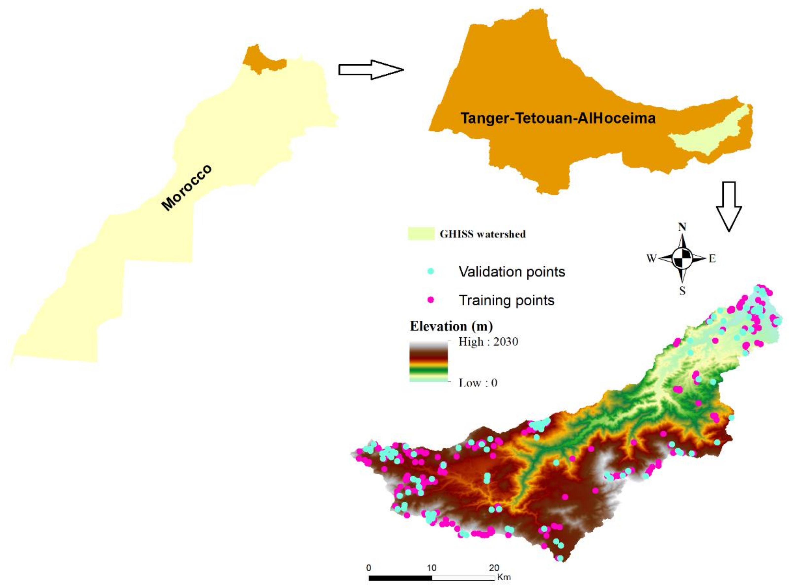
2.1. Study Area
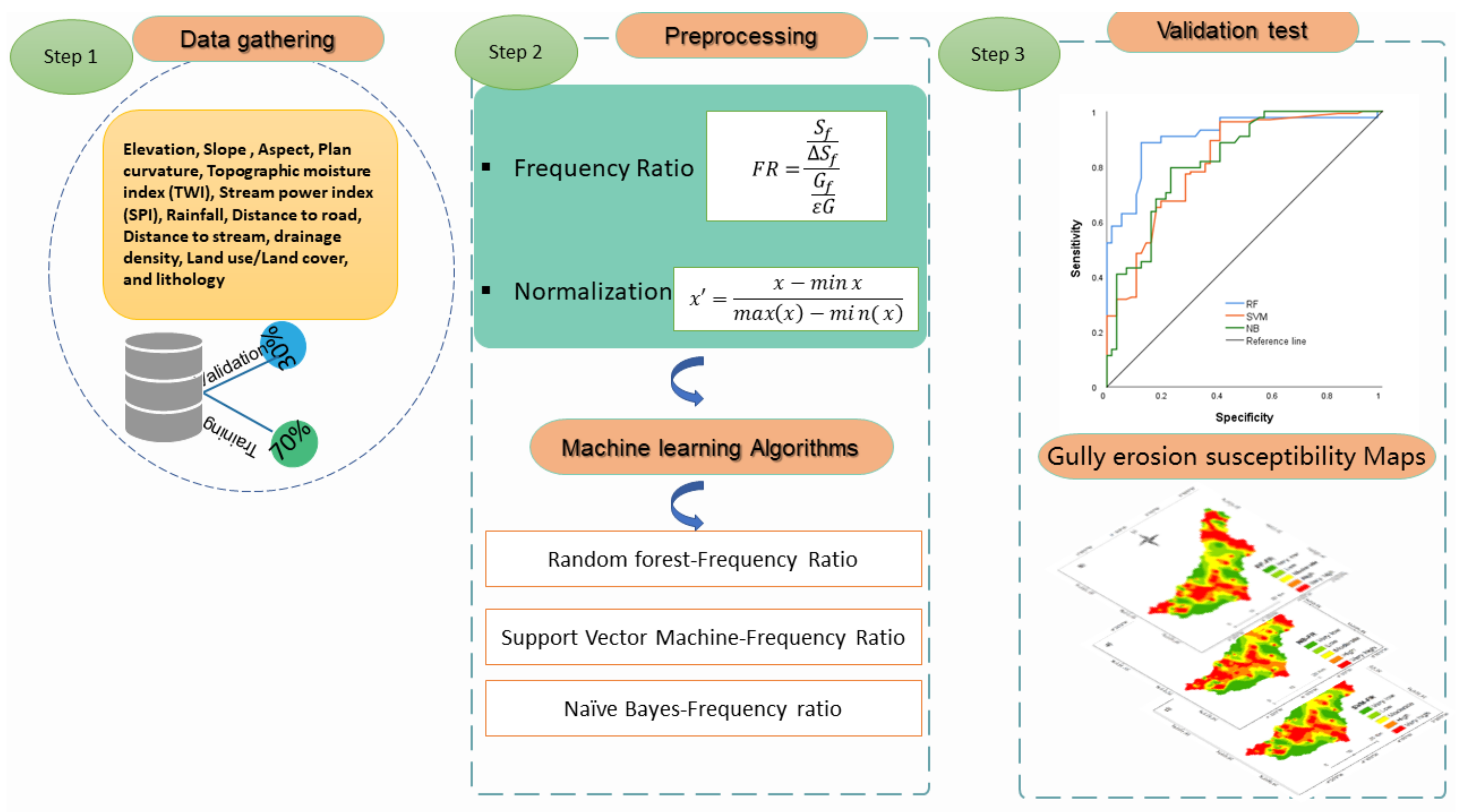
2.2. Data Used and Methodology
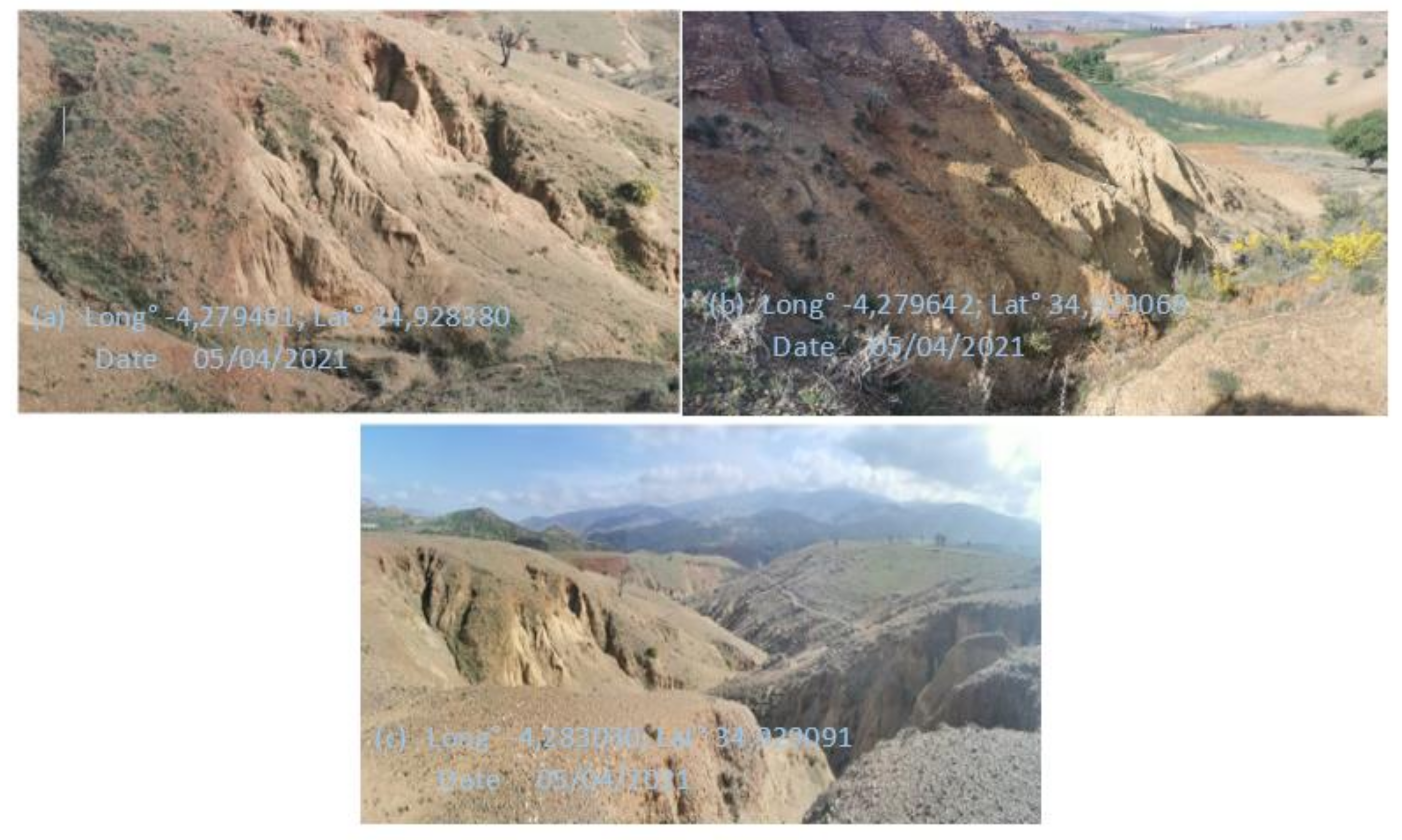
2.3. Gully Erosion Inventory Map
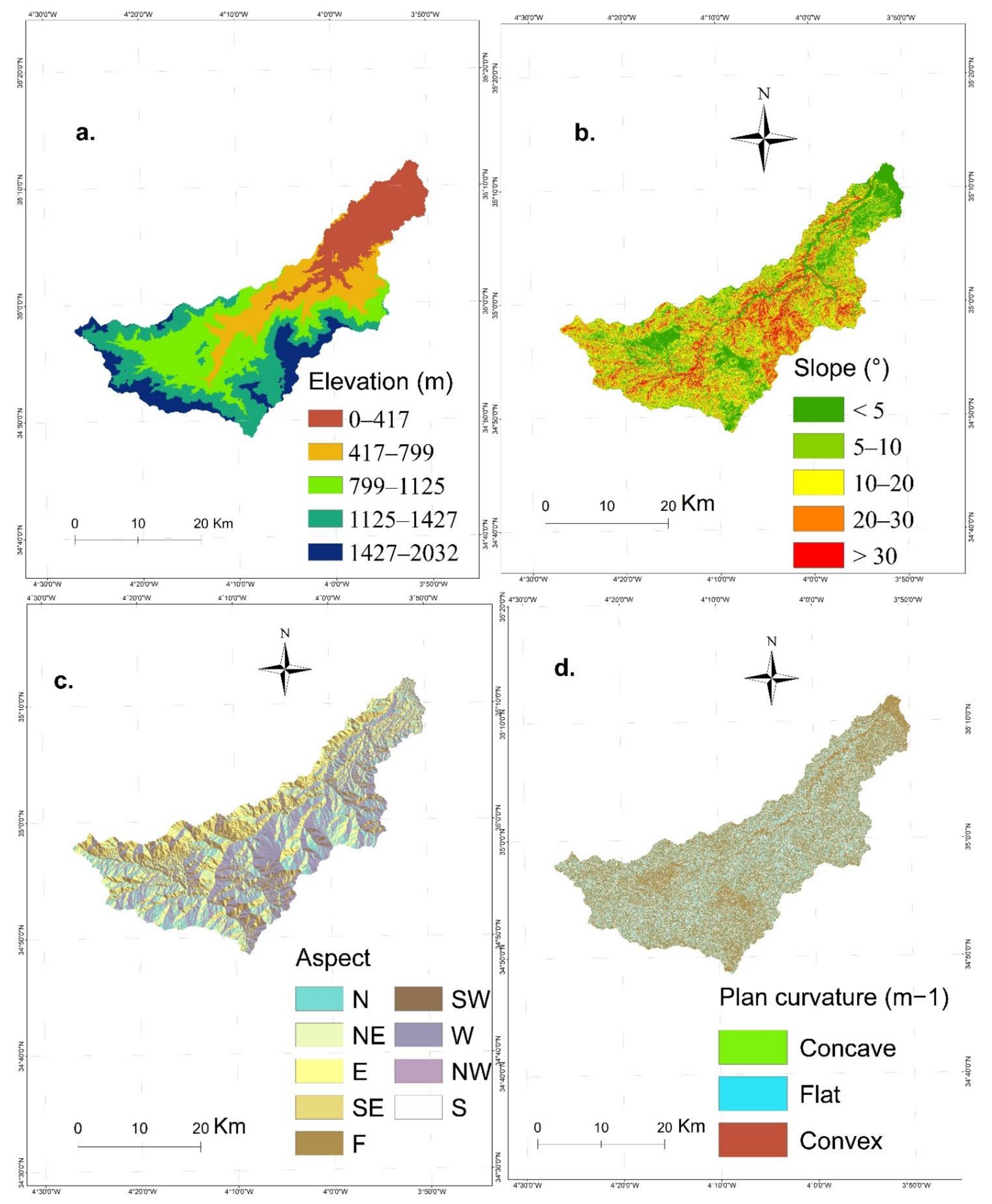
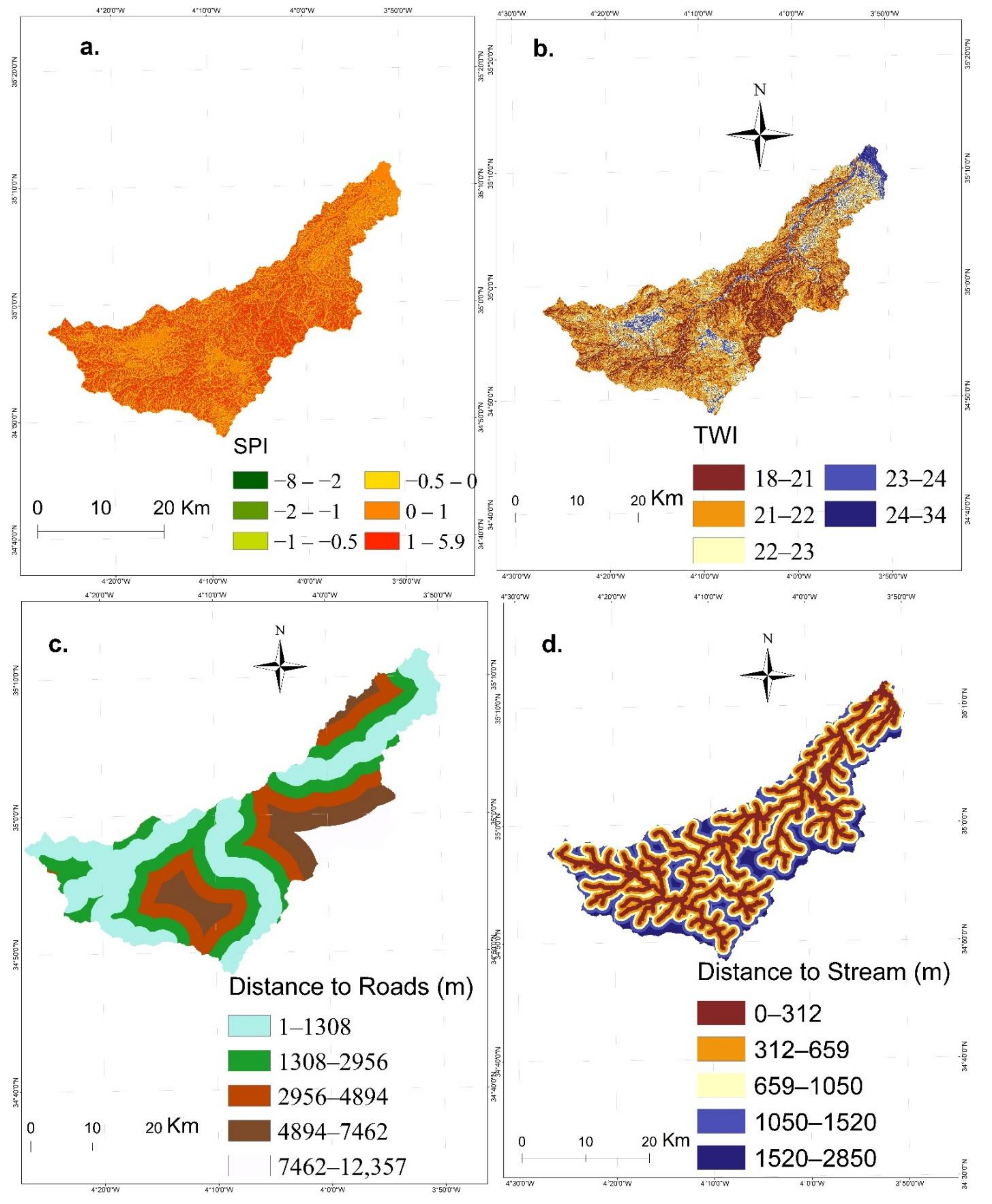
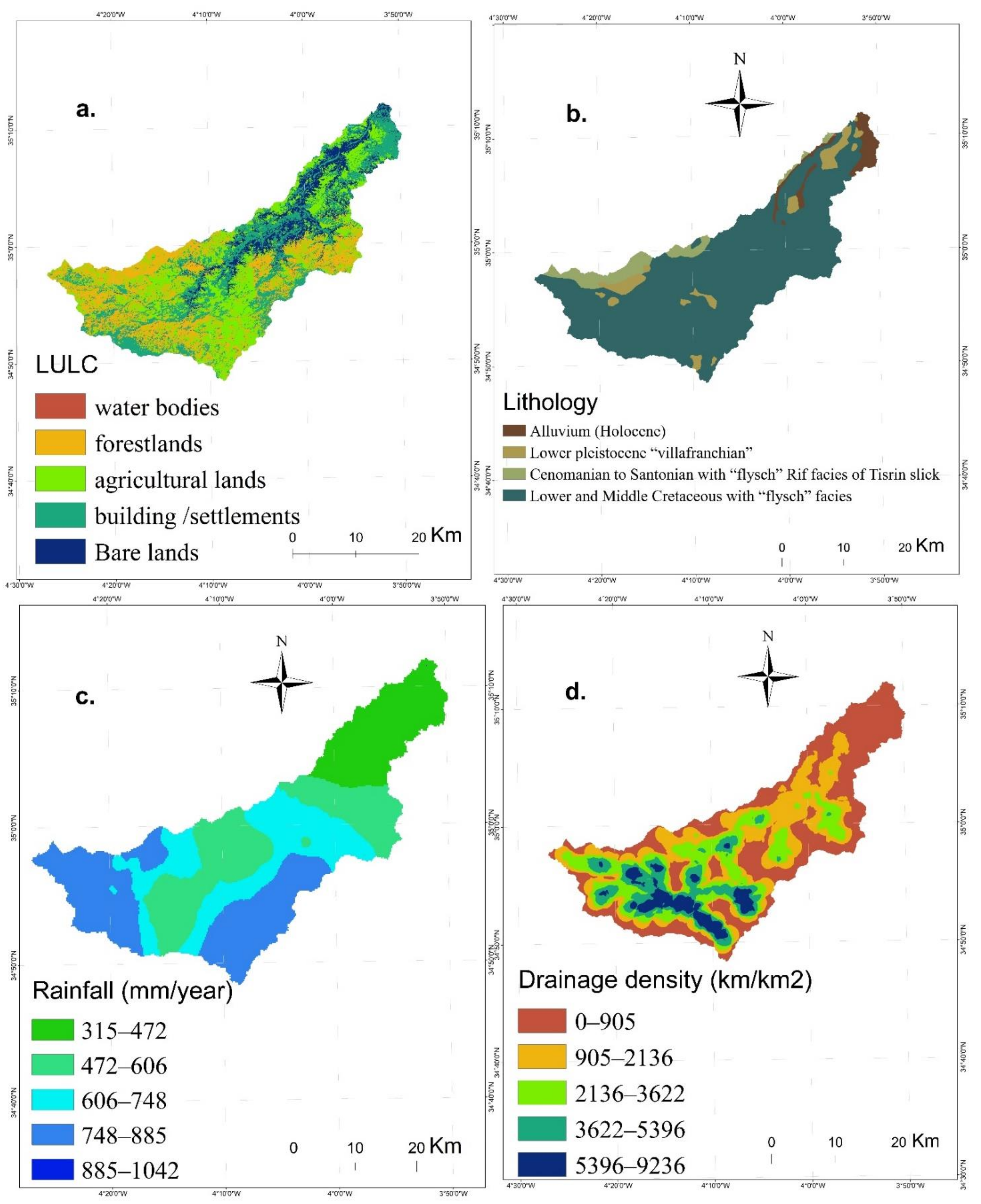
2.4. Parameters’ Description
2.5. Multicollinearity Analysis
3. Models and Methods Background
3.1. Frequency Ratio (FR)
3.2. Random Forest (RF)
3.3. Support Vector Machine (SVM)
3.4. Naïve Bayes (NB)
3.5. Model Validation
3.6. Variable Importance Using Information Gain Index
4. Results
4.1. Results of Frequency Ratio
4.2. Results of Multicollinearity Assessment
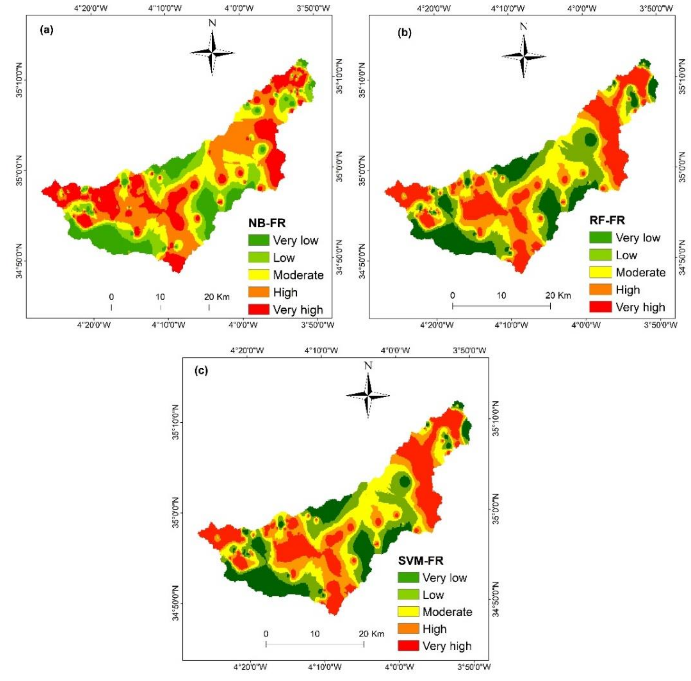
4.3. Identification of Gully Zones
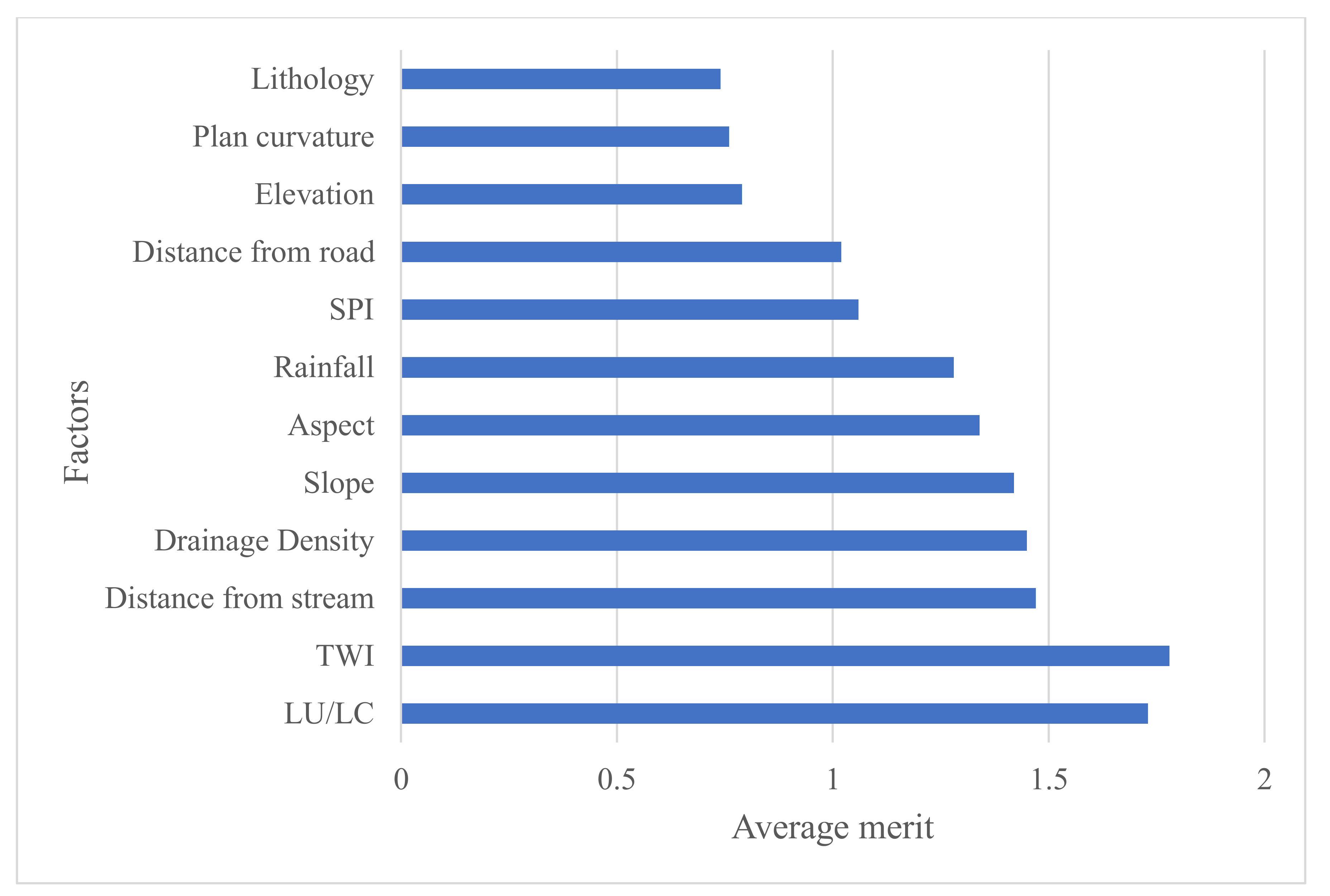
4.4. Variable Importance
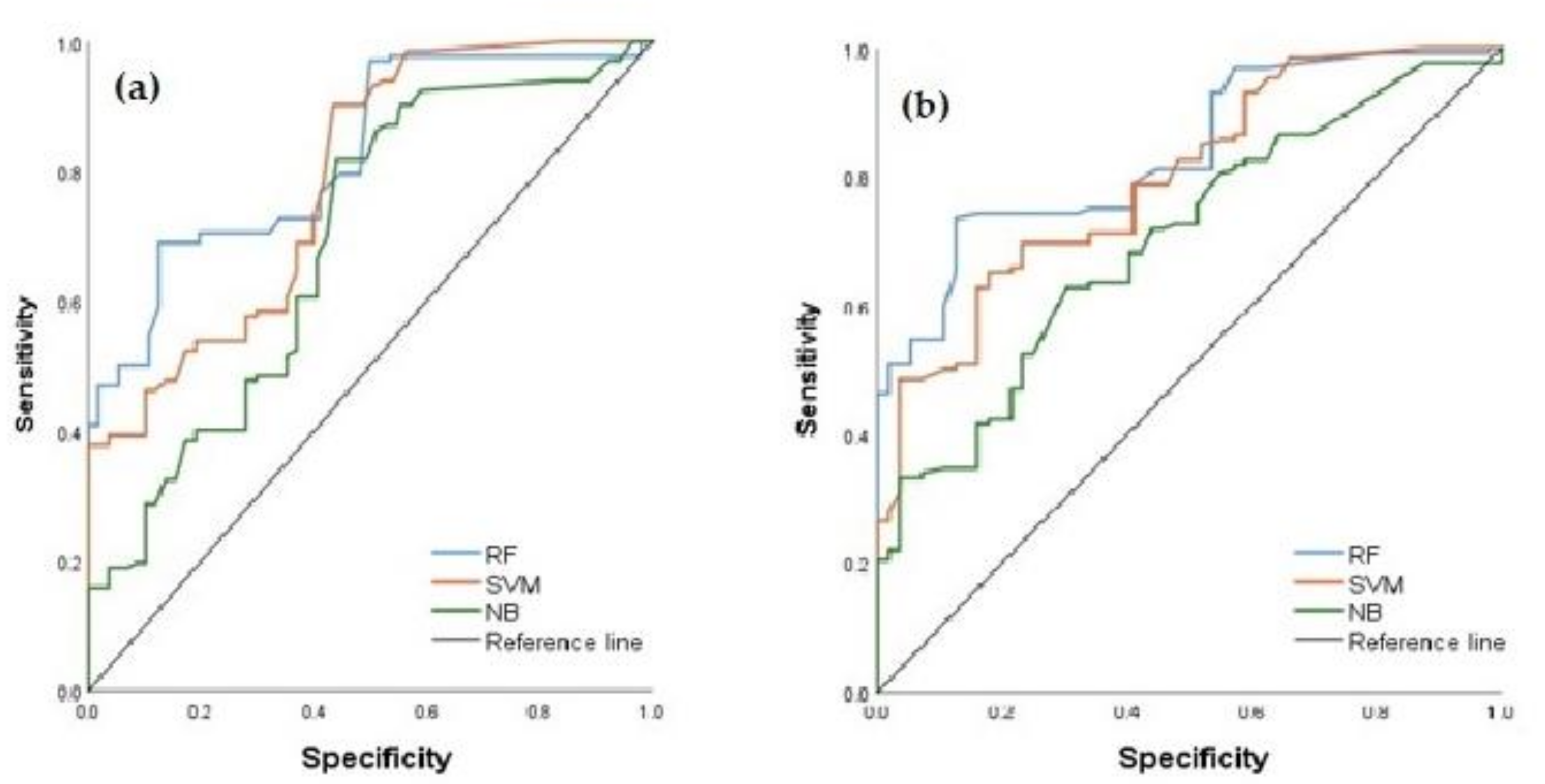
4.5. Validation of Gully Erosion Models
5. Discussion
6. Conclusions
Author Contributions
Funding
Institutional Review Board Statement
Informed Consent Statement
Data Availability Statement
Conflicts of Interest
References
- Domazetović, F.; Šiljeg, A.; Lončar, N.; Marić, I. Development of Automated Multicriteria GIS Analysis of Gully Erosion Susceptibility. Appl. Geogr. 2019, 112, 102083. [Google Scholar] [CrossRef]
- Fadul, H.M.; Salih, A.A.; Ali, I.A.; Inanaga, S. Use of Remote Sensing to Map Gully Erosion along the Atbara River, Sudan. Int. J. Appl. Earth Obs. Geoinf. 1999, 1, 175–180. [Google Scholar] [CrossRef]
- Magliulo, P. Assessing the Susceptibility to Water-Induced Soil Erosion Using a Geomorphological, Bivariate Statistics-Based Approach. Environ. Earth Sci. 2012, 67, 1801–1820. [Google Scholar] [CrossRef]
- Dooley, E.; Roberts, E.; Wunder, S. Land Degradation Neutrality under the SDGs: National and International Implementation of the Land Degradation Neutral World Target. Elni. Rev. 2015, 1, 2–9. [Google Scholar] [CrossRef]
- Safriel, U. Land Degradation Neutrality (LDN) in Drylands and beyond—Where Has It Come from and Where Does It Go. Silva Fenn. 2017, 51, 20–24. [Google Scholar] [CrossRef] [Green Version]
- Durán Zuazo, V.H.; Rodríguez Pleguezuelo, C.R. Soil-Erosion and Runoff Prevention by Plant Covers. A Review. Agron. Sustain. Dev. 2008, 28, 65–86. [Google Scholar] [CrossRef] [Green Version]
- Lal, R. Soil Erosion Impact on Agronomic Productivity and Environment Quality. Crit. Rev. Plant Sci. 1998, 17, 319–464. [Google Scholar] [CrossRef]
- Peter, K.D.; d’Oleire-Oltmanns, S.; Ries, J.B.; Marzolff, I.; Ait Hssaine, A. Soil Erosion in Gully Catchments Affected by Land-Levelling Measures in the Souss Basin, Morocco, Analysed by Rainfall Simulation and UAV Remote Sensing Data. CATENA 2014, 113, 24–40. [Google Scholar] [CrossRef]
- Simonneaux, V.; Cheggour, A.; Deschamps, C.; Mouillot, F.; Cerdan, O.; Le Bissonnais, Y. Land Use and Climate Change Effects on Soil Erosion in a Semi-Arid Mountainous Watershed (High Atlas, Morocco). J. Arid Environ. 2015, 122, 64–75. [Google Scholar] [CrossRef] [Green Version]
- Azedou, A.; Lahssini, S.; Khattabi, A.; Meliho, M.; Rifai, N. A Methodological Comparison of Three Models for Gully Erosion Susceptibility Mapping in the Rural Municipality of El Faid (Morocco). Sustainability 2021, 13, 682. [Google Scholar] [CrossRef]
- Tairi, A.; Elmouden, A.; Bouchaou, L.; Aboulouafa, M. Mapping Soil Erosion–Prone Sites through GIS and Remote Sensing for the Tifnout Askaoun Watershed, Southern Morocco. Arab. J. Geosci. 2021, 14, 811. [Google Scholar] [CrossRef]
- Kachouri, S.; Achour, H.; Abida, H.; Bouaziz, S. Soil Erosion Hazard Mapping Using Analytic Hierarchy Process and Logistic Regression: A Case Study of Haffouz Watershed, Central Tunisia. Arab. J. Geosci. 2015, 8, 4257–4268. [Google Scholar] [CrossRef]
- Saha, S.; Gayen, A.; Pourghasemi, H.R.; Tiefenbacher, J.P. Identification of Soil Erosion-Susceptible Areas Using Fuzzy Logic and Analytical Hierarchy Process Modeling in an Agricultural Watershed of Burdwan District, India. Environ. Earth Sci. 2019, 78, 649. [Google Scholar] [CrossRef]
- Senouci, R.; Taibi, N.-E.; Teodoro, A.C.; Duarte, L.; Mansour, H.; Yahia Meddah, R. GIS-Based Expert Knowledge for Landslide Susceptibility Mapping (LSM): Case of Mostaganem Coast District, West of Algeria. Sustainability 2021, 13, 630. [Google Scholar] [CrossRef]
- Senanayake, S.; Pradhan, B.; Huete, A.; Brennan, J. Assessing Soil Erosion Hazards Using Land-Use Change and Landslide Frequency Ratio Method: A Case Study of Sabaragamuwa Province, Sri Lanka. Remote Sens. 2020, 12, 1483. [Google Scholar] [CrossRef]
- Tehrany, M.S.; Shabani, F.; Javier, D.N.; Kumar, L. Soil Erosion Susceptibility Mapping for Current and 2100 Climate Conditions Using Evidential Belief Function and Frequency Ratio. Geomat. Nat. Hazards Risk 2017, 8, 1695–1714. [Google Scholar] [CrossRef] [Green Version]
- Arabameri, A.; Pradhan, B.; Rezaei, K. Gully Erosion Zonation Mapping Using Integrated Geographically Weighted Regression with Certainty Factor and Random Forest Models in GIS. J. Environ. Manage. 2019, 232, 928–942. [Google Scholar] [CrossRef]
- Azareh, A.; Rahmati, O.; Rafiei-Sardooi, E.; Sankey, J.B.; Lee, S.; Shahabi, H.; Ahmad, B.B. Modelling Gully-Erosion Susceptibility in a Semi-Arid Region, Iran: Investigation of Applicability of Certainty Factor and Maximum Entropy Models. Sci. Total Environ. 2019, 655, 684–696. [Google Scholar] [CrossRef]
- Hembram, T.K.; Paul, G.C.; Saha, S. Comparative Analysis between Morphometry and Geo-Environmental Factor Based Soil Erosion Risk Assessment Using Weight of Evidence Model: A Study on Jainti River Basin, Eastern India. Environ. Process. 2019, 6, 883–913. [Google Scholar] [CrossRef]
- Meliho, M.; Khattabi, A.; Mhammdi, N. A GIS-Based Approach for Gully Erosion Susceptibility Modelling Using Bivariate Statistics Methods in the Ourika Watershed, Morocco. Environ. Earth Sci. 2018, 77, 655. [Google Scholar] [CrossRef]
- Pourghasemi, H.R.; Mohammady, M.; Pradhan, B. Landslide Susceptibility Mapping Using Index of Entropy and Conditional Probability Models in GIS: Safarood Basin, Iran. CATENA 2012, 97, 71–84. [Google Scholar] [CrossRef]
- Pournader, M.; Ahmadi, H.; Feiznia, S.; Karimi, H.; Peirovan, H.R. Spatial Prediction of Soil Erosion Susceptibility: An Evaluation of the Maximum Entropy Model. Earth Sci. Inform. 2018, 11, 389–401. [Google Scholar] [CrossRef]
- Nosrati, K. Assessing Soil Quality Indicator under Different Land Use and Soil Erosion Using Multivariate Statistical Techniques. Environ. Monit. Assess. 2013, 185, 2895–2907. [Google Scholar] [CrossRef] [PubMed]
- Sarkar, T.; Mishra, M. Soil Erosion Susceptibility Mapping with the Application of Logistic Regression and Artificial Neural Network. J. Geovisualization Spat. Anal. 2018, 2, 8. [Google Scholar] [CrossRef]
- Gholami, V.; Sahour, H.; Hadian Amri, M.A. Soil Erosion Modeling Using Erosion Pins and Artificial Neural Networks. CATENA 2021, 196, 104902. [Google Scholar] [CrossRef]
- Gholami, V.; Booij, M.J.; Nikzad Tehrani, E.; Hadian, M.A. Spatial Soil Erosion Estimation Using an Artificial Neural Network (ANN) and Field Plot Data. CATENA 2018, 163, 210–218. [Google Scholar] [CrossRef]
- Dinh, T.V.; Nguyen, H.; Tran, X.-L.; Hoang, N.-D. Predicting Rainfall-Induced Soil Erosion Based on a Hybridization of Adaptive Differential Evolution and Support Vector Machine Classification. Math. Probl. Eng. 2021, 2021, 6647829. [Google Scholar] [CrossRef]
- Arabameri, A.; Asadi Nalivan, O.; Chandra Pal, S.; Chakrabortty, R.; Saha, A.; Lee, S.; Pradhan, B.; Tien Bui, D. Novel Machine Learning Approaches for Modelling the Gully Erosion Susceptibility. Remote Sens. 2020, 12, 2833. [Google Scholar] [CrossRef]
- Ghosh, A.; Maiti, R. Soil Erosion Susceptibility Assessment Using Logistic Regression, Decision Tree and Random Forest: Study on the Mayurakshi River Basin of Eastern India. Environ. Earth Sci. 2021, 80, 328. [Google Scholar] [CrossRef]
- Phinzi, K.; Ngetar, N.S.; Ebhuoma, O. Soil Erosion Risk Assessment in the Umzintlava Catchment (T32E), Eastern Cape, South Africa, Using RUSLE and Random Forest Algorithm. S. Afr. Geogr. J. 2021, 103, 139–162. [Google Scholar] [CrossRef]
- Choubin, B.; Moradi, E.; Golshan, M.; Adamowski, J.; Sajedi-Hosseini, F.; Mosavi, A. An Ensemble Prediction of Flood Susceptibility Using Multivariate Discriminant Analysis, Classification and Regression Trees, and Support Vector Machines. Sci. Total Environ. 2019, 651, 2087–2096. [Google Scholar] [CrossRef]
- Lee, S.; Lee, M.-J.; Jung, H.-S.; Lee, S. Landslide Susceptibility Mapping Using Naïve Bayes and Bayesian Network Models in Umyeonsan, Korea. Geocarto Int. 2020, 35, 1665–1679. [Google Scholar] [CrossRef]
- Mosavi, A.; Sajedi-Hosseini, F.; Choubin, B.; Taromideh, F.; Rahi, G.; Dineva, A. Susceptibility Mapping of Soil Water Erosion Using Machine Learning Models. Water 2020, 12, 1995. [Google Scholar] [CrossRef]
- Lei, X.; Chen, W.; Avand, M.; Janizadeh, S.; Kariminejad, N.; Shahabi, H.; Costache, R.; Shahabi, H.; Shirzadi, A.; Mosavi, A. GIS-Based Machine Learning Algorithms for Gully Erosion Susceptibility Mapping in a Semi-Arid Region of Iran. Remote Sens. 2020, 12, 2478. [Google Scholar] [CrossRef]
- Saha, S.; Roy, J.; Arabameri, A.; Blaschke, T.; Tien Bui, D. Machine Learning-Based Gully Erosion Susceptibility Mapping: A Case Study of Eastern India. Sensors 2020, 20, 1313. [Google Scholar] [CrossRef] [Green Version]
- Gayen, A.; Pourghasemi, H.R.; Saha, S.; Keesstra, S.; Bai, S. Gully Erosion Susceptibility Assessment and Management of Hazard-Prone Areas in India Using Different Machine Learning Algorithms. Sci. Total Environ. 2019, 668, 124–138. [Google Scholar] [CrossRef]
- Pal, S.C.; Arabameri, A.; Blaschke, T.; Chowdhuri, I.; Saha, A.; Chakrabortty, R.; Lee, S.; Band, S.S. Ensemble of Machine-Learning Methods for Predicting Gully Erosion Susceptibility. Remote Sens. 2020, 12, 3675. [Google Scholar] [CrossRef]
- Soleimanpour, S.M.; Pourghasemi, H.R.; Zare, M. A Comparative Assessment of Gully Erosion Spatial Predictive Modeling Using Statistical and Machine Learning Models. CATENA 2021, 207, 105679. [Google Scholar] [CrossRef]
- Razavi-Termeh, S.V.; Sadeghi-Niaraki, A.; Choi, S.-M. Gully Erosion Susceptibility Mapping Using Artificial Intelligence and Statistical Models. Geomat. Nat. Hazards Risk 2020, 11, 821–844. [Google Scholar] [CrossRef]
- Pourghasemi, H.R.; Sadhasivam, N.; Kariminejad, N.; Collins, A.L. Gully Erosion Spatial Modelling: Role of Machine Learning Algorithms in Selection of the Best Controlling Factors and Modelling Process. Geosci. Front. 2020, 11, 2207–2219. [Google Scholar] [CrossRef]
- Avand, J.; Janizadeh, S.; Naghibi, S.A.; Pourghasemi, H.R.; Bozchaloei, S.K.; Blaschke, T. A Comparative Assessment of Random Forest and K-Nearest Neighbor Classifiers for Gully Erosion Susceptibility Mapping. Water 2019, 11, 2076. [Google Scholar] [CrossRef] [Green Version]
- Pham, Q.B.; Mukherjee, K.; Norouzi, A.; Linh, N.T.T.; Janizadeh, S.; Ahmadi, K.; Cerdà, A.; Doan, T.N.C.; Anh, D.T. Head-Cut Gully Erosion Susceptibility Modelling Based on Ensemble Random Forest with Oblique Decision Trees in Fareghan Watershed, Iran. Geomat. Nat. Hazards Risk 2020, 11, 2385–2410. [Google Scholar] [CrossRef]
- Arabameri, A.; Chen, W.; Lombardo, L.; Blaschke, T.; Tien Bui, D. Hybrid Computational Intelligence Models for Improvement Gully Erosion Assessment. Remote Sens. 2020, 12, 140. [Google Scholar] [CrossRef] [Green Version]
- Ahmadpour, H.; Bazrafshan, O.; Rafiei-Sardooi, E.; Zamani, H.; Panagopoulos, T. Gully Erosion Susceptibility Assessment in the Kondoran Watershed Using Machine Learning Algorithms and the Boruta Feature Selection. Sustainability 2021, 13, 10110. [Google Scholar] [CrossRef]
- Chen, Y.; Chen, W.; Janizadeh, S.; Bhunia, G.S.; Bera, A.; Pham, Q.B.; Linh, N.T.T.; Balogun, A.-L.; Wang, X. Deep Learning and Boosting Framework for Piping Erosion Susceptibility Modeling: Spatial Evaluation of Agricultural Areas in the Semi-Arid Region. Geocarto. Int. 2021, 12, 1–27. [Google Scholar] [CrossRef]
- Yang, A.; Wang, C.; Pang, G.; Long, Y.; Wang, L.; Cruse, R.M.; Yang, Q. Gully Erosion Susceptibility Mapping in Highly Complex Terrain Using Machine Learning Models. ISPRS Int. J. Geo-Inf. 2021, 10, 680. [Google Scholar] [CrossRef]
- Saha, S.; Sarkar, R.; Thapa, G.; Roy, J. Modeling Gully Erosion Susceptibility in Phuentsholing, Bhutan Using Deep Learning and Basic Machine Learning Algorithms. Environ. Earth Sci. 2021, 80, 295. [Google Scholar] [CrossRef]
- Kadavi, P.; Lee, C.-W.; Lee, S. Application of Ensemble-Based Machine Learning Models to Landslide Susceptibility Mapping. Remote Sens. 2018, 10, 1252. [Google Scholar] [CrossRef] [Green Version]
- Lee, S.; Pradhan, B. Probabilistic Landslide Hazards and Risk Mapping on Penang Island, Malaysia. J. Earth Syst. Sci. 2006, 115, 661–672. [Google Scholar] [CrossRef]
- Costache, R.; Ngo, P.T.T.; Bui, D.T. Novel Ensembles of Deep Learning Neural Network and Statistical Learning for Flash-Flood Susceptibility Mapping. Water 2020, 12, 1549. [Google Scholar] [CrossRef]
- Ijlil, S.; Essahlaoui, A.; Mohajane, M.; Essahlaoui, N.; Mili, E.M.; Van Rompaey, A. Machine Learning Algorithms for Modeling and Mapping of Groundwater Pollution Risk: A Study to Reach Water Security and Sustainable Development (Sdg) Goals in a Mediterranean Aquifer System. Remote Sens. 2022, 14, 2379. [Google Scholar] [CrossRef]
- Arabameri, A.; Cerda, A.; Rodrigo-Comino, J.; Pradhan, B.; Sohrabi, M.; Blaschke, T.; Bui, D.T. Proposing a Novel Predictive Technique for Gully Erosion Susceptibility Mapping in Arid and Semi-Arid Regions (Iran). Remote Sens. 2019, 11, 2577. [Google Scholar] [CrossRef] [Green Version]
- Bouamrane, A.; Bouamrane, A.; Abida, H. Water Erosion Hazard Distribution under a Semi-Arid Climate Condition: Case of Mellah Watershed, North-Eastern Algeria. Geoderma 2021, 403, 115381. [Google Scholar] [CrossRef]
- Nouayti, N.; Cherif, E.K.; Algarra, M.; Pola, M.L.; Fernández, S.; Nouayti, A.; Esteves da Silva, J.C.G.; Driss, K.; Samlani, N.; Mohamed, H.; et al. Determination of Physicochemical Water Quality of the Ghis-Nekor Aquifer (Al Hoceima, Morocco) Using Hydrochemistry, Multiple Isotopic Tracers, and the Geographical Information System (GIS). Water 2022, 14, 606. [Google Scholar] [CrossRef]
- Bouhout, S.; Haboubi, K.; Zian, A.; Elyoubi, M.S.; Elabdouni, A. Evaluation of Two Linear Kriging Methods for Piezometric Levels Interpolation and a Framework for Upgrading Groundwater Level Monitoring Network in Ghiss-Nekor Plain, North-Eastern Morocco. Arab. J. Geosci. 2022, 15, 1016. [Google Scholar] [CrossRef]
- Benabdelouahab, S.; Salhi, A.; Stitou, J.; Himi, M.; Draoui, M.; Casas, A. Application Des SIG et de La Tomographie Électrique Pour Contribuer à La Protection de l’aquifère de Martil-Alila (Maroc). In Proceedings of the Euromediterranean Scientific Congress on Engineering, Algeciras, Spain, 19–20 May 2011. [Google Scholar]
- Bourjila, A.; Dimane, F.; EL Ouarghi, H.; Nouayti, N.; Taher, M.; EL Hammoudani, Y.; Saadi, O.; Bensiali, A. Groundwater Potential Zones Mapping by Applying GIS, Remote Sensing and Multi-Criteria Decision Analysis in the Ghiss Basin, Northern Morocco. Groundw. Sustain. Dev. 2021, 15, 100693. [Google Scholar] [CrossRef]
- El Motaki, H.; El-Fengour, A.; Aissa, E.; Madureira, H.; Monteiro, A. The Global Change Impacts on Forest Natural Resources in Central Rif Mountains in Northern Morocco: Extensive Exploration and Planning Perspective. GOT—J. Geogr. Spat. Plan. 2019, 17, 75–92. [Google Scholar] [CrossRef]
- Leikine, M.; Asebriy, L.; Bourgois, J. About the Age of the Ketama Unit’s Anchi-Epizonal Metamorphism, Central Rif, Morocco. Comptes Rendus—Acad. Sci. Ser. II 1991, 313, 787–793. [Google Scholar]
- Mansour, S.; Kouz, T.; Thaiki, M.; Ouhadi, A.; Mesmoudi, H.; Hassani Zerrouk, M.; Mourabit, T.; Dakak, H.; Cherkaoui Dekkaki, H. Spatial Assessment of the Vulnerability of Water Resources against Anthropogenic Pollution Using the DKPR Model: A Case of Ghiss-Nekkour Basin, Morocco. Arab. J. Geosci. 2021, 14, 699. [Google Scholar] [CrossRef]
- Benyoussef, S.; Arabi, M.; El Ouarghi, H.; Ghalit, M.; Azirar, M.; El Midaoui, A.; Ait Boughrous, A. Impact of Anthropic Activities on the Quality of Groundwater in the Central Rif (North Morocco). Ecol. Eng. Environ. Technol. 2021, 22, 69–78. [Google Scholar] [CrossRef]
- Taher, M.; Mourabit, T.; Bourjila, A.; Saadi, O.; Errahmouni, A.; El Marzkioui, F.; El Mousaoui, M. An Estimation of Soil Erosion Rate Hot Spots by Integrated USLE and GIS Methods: A Case Study of the Ghiss Dam and Basin in Northeastern Morocco. Geomat. Environ. Eng. 2022, 16, 95–110. [Google Scholar] [CrossRef]
- Tsangaratos, P.; Ilia, I.; Hong, H.; Chen, W.; Xu, C. Applying Information Theory and GIS-Based Quantitative Methods to Produce Landslide Susceptibility Maps in Nancheng County, China. Landslides 2017, 14, 1091–1111. [Google Scholar] [CrossRef]
- Amiri, M.; Pourghasemi, H.R.; Ghanbarian, G.A.; Afzali, S.F. Assessment of the Importance of Gully Erosion Effective Factors Using Boruta Algorithm and Its Spatial Modeling and Mapping Using Three Machine Learning Algorithms. Geoderma 2019, 340, 55–69. [Google Scholar] [CrossRef]
- Valentin, C.; Poesen, J.; Li, Y. Gully Erosion: Impacts, Factors and Control. CATENA 2005, 63, 132–153. [Google Scholar] [CrossRef]
- Hembram, T.K.; Paul, G.C.; Saha, S. Modelling of Gully Erosion Risk Using New Ensemble of Conditional Probability and Index of Entropy in Jainti River Basin of Chotanagpur Plateau Fringe Area, India. Appl. Geomat. 2020, 12, 337–360. [Google Scholar] [CrossRef]
- Conforti, M.; Aucelli, P.P.C.; Robustelli, G.; Scarciglia, F. Geomorphology and GIS Analysis for Mapping Gully Erosion Susceptibility in the Turbolo Stream Catchment (Northern Calabria, Italy). Nat. Hazards 2011, 56, 881–898. [Google Scholar] [CrossRef]
- Arabameri, A.; Chandra Pal, S.; Costache, R.; Saha, A.; Rezaie, F.; Seyed Danesh, A.; Pradhan, B.; Lee, S.; Hoang, N.-D. Prediction of Gully Erosion Susceptibility Mapping Using Novel Ensemble Machine Learning Algorithms. Geomat. Nat. Hazards Risk 2021, 12, 469–498. [Google Scholar] [CrossRef]
- Moore, I.D.; Grayson, R.B.; Ladson, A.R. Digital Terrain Modelling: A Review of Hydrological, Geomorphological, and Biological Applications. Hydrol. Process. 1991, 5, 3–30. [Google Scholar] [CrossRef]
- Band, S.S.; Janizadeh, S.; Chandra Pal, S.; Saha, A.; Chakrabortty, R.; Shokri, M.; Mosavi, A. Novel Ensemble Approach of Deep Learning Neural Network (DLNN) Model and Particle Swarm Optimization (PSO) Algorithm for Prediction of Gully Erosion Susceptibility. Sensors 2020, 20, 5609. [Google Scholar] [CrossRef]
- Chowdhuri, I.; Pal, S.C.; Saha, A.; Chakrabortty, R.; Roy, P. Evaluation of Different DEMs for Gully Erosion Susceptibility Mapping Using In-Situ Field Measurement and Validation. Ecol. Inform. 2021, 65, 101425. [Google Scholar] [CrossRef]
- Bui, D.T.; Lofman, O.; Revhaug, I.; Dick, O. Landslide Susceptibility Analysis in the Hoa Binh Province of Vietnam Using Statistical Index and Logistic Regression. Nat. Hazards 2011, 59, 1413–1444. [Google Scholar] [CrossRef]
- Rahmati, O.; Pourghasemi, H.R.; Zeinivand, H. Flood Susceptibility Mapping Using Frequency Ratio and Weights-of-Evidence Models in the Golastan Province, Iran. Geocarto Int. 2016, 31, 42–70. [Google Scholar] [CrossRef]
- Lee, S.; Sambath, T. Landslide Susceptibility Mapping in the Damrei Romel Area, Cambodia Using Frequency Ratio and Logistic Regression Models. Environ. Geol. 2006, 50, 847–855. [Google Scholar] [CrossRef]
- Samanta, R.K.; Bhunia, G.S.; Shit, P.K.; Pourghasemi, H.R. Flood Susceptibility Mapping Using Geospatial Frequency Ratio Technique: A Case Study of Subarnarekha River Basin, India. Model. Earth Syst. Environ. 2018, 4, 395–408. [Google Scholar] [CrossRef]
- Mohajane, M.; Costache, R.; Karimi, F.; Bao Pham, Q.; Essahlaoui, A.; Nguyen, H.; Laneve, G.; Oudija, F. Application of Remote Sensing and Machine Learning Algorithms for Forest Fire Mapping in a Mediterranean Area. Ecol. Indic. 2021, 129, 107869. [Google Scholar] [CrossRef]
- Boroughani, M.; Pourhashemi, S.; Hashemi, H.; Salehi, M.; Amirahmadi, A.; Asadi, M.A.Z.; Berndtsson, R. Application of Remote Sensing Techniques and Machine Learning Algorithms in Dust Source Detection and Dust Source Susceptibility Mapping. Ecol. Inform. 2020, 56, 101059. [Google Scholar] [CrossRef]
- Breiman, L. Random Forests Machine Learning. Kluwer Academic Publishers: Dordrecht, The Netherlands, 2001; Volume 45. [Google Scholar]
- Ho, T.K. The Random Subspace Method for Constructing Decision Forests. IEEE Trans. Pattern Anal. Mach. Intell. 1998, 20, 832–844. [Google Scholar] [CrossRef] [Green Version]
- Rodriguez-Galiano, V.F.; Chica-Olmo, M.; Chica-Rivas, M. Predictive Modelling of Gold Potential with the Integration of Multisource Information Based on Random Forest: A Case Study on the Rodalquilar Area, Southern Spain. Int. J. Geogr. Inf. Sci. 2014, 28, 1336–1354. [Google Scholar] [CrossRef]
- Arabameri, A.; Pradhan, B.; Rezaei, K. Spatial Prediction of Gully Erosion Using ALOS PALSAR Data and Ensemble Bivariate and Data Mining Models. Geosci. J. 2019, 23, 669–686. [Google Scholar] [CrossRef]
- Pai, P.-F.; Hsu, M.-F. An Enhanced Support Vector Machines Model for Classification and Rule Generation. In Computational Optimization, Methods and Algorithms; Koziel, S., Yang, X.-S., Eds.; Studies in Computational Intelligence; Springer: Berlin/Heidelberg, Germany, 2011; Volume 356, pp. 241–258, ISBN 978-3-642-20858-4. [Google Scholar]
- Rahmati, O.; Tahmasebipour, N.; Haghizadeh, A.; Pourghasemi, H.R.; Feizizadeh, B. Evaluation of Different Machine Learning Models for Predicting and Mapping the Susceptibility of Gully Erosion. Geomorphology 2017, 298, 118–137. [Google Scholar] [CrossRef]
- Garosi, Y.; Sheklabadi, M.; Conoscenti, C.; Pourghasemi, H.R.; Van Oost, K. Assessing the Performance of GIS- Based Machine Learning Models with Different Accuracy Measures for Determining Susceptibility to Gully Erosion. Sci. Total Environ. 2019, 664, 1117–1132. [Google Scholar] [CrossRef]
- Phinzi, K.; Abriha, D.; Bertalan, L.; Holb, I.; Szabó, S. Machine Learning for Gully Feature Extraction Based on a Pan-Sharpened Multispectral Image: Multiclass vs. Binary Approach. ISPRS Int. J. Geo-Inf. 2020, 9, 252. [Google Scholar] [CrossRef] [Green Version]
- Ranjitha, K.V. Classification and Optimization Scheme for Text Data Using Machine Learning Naïve Bayes Classifier. In Proceedings of the 2018 IEEE World Symposium on Communication Engineering (WSCE), Singapore, 28–30 December 2018; IEEE: Singapore, 2018; pp. 33–36. [Google Scholar]
- Serrano-Cinca, C.; Gutiérrez-Nieto, B. Partial Least Square Discriminant Analysis for Bankruptcy Prediction. Decis. Support Syst. 2013, 54, 1245–1255. [Google Scholar] [CrossRef]
- Pourghasemi, H.; Gayen, A.; Park, S.; Lee, C.-W.; Lee, S. Assessment of Landslide-Prone Areas and Their Zonation Using Logistic Regression, LogitBoost, and NaïveBayes Machine-Learning Algorithms. Sustainability 2018, 10, 3697. [Google Scholar] [CrossRef] [Green Version]
- Bhargavi, P.; Tech, M.; Jyothi, D.S. Applying Naive Bayes Data Mining Technique for Classification of Agricultural Land Soils. Int. J. Comput. Sci. Netw. Secur. 2009, 6, 189–193. [Google Scholar]
- Pham, B.T.; Jaafari, A.; Avand, M.; Al-Ansari, N.; Dinh Du, T.; Yen, H.P.H.; Phong, T.V.; Nguyen, D.H.; Le, H.V.; Mafi-Gholami, D.; et al. Performance Evaluation of Machine Learning Methods for Forest Fire Modeling and Prediction. Symmetry 2020, 12, 1022. [Google Scholar] [CrossRef]
- Domazetović, F.; Šiljeg, A.; Lončar, N.; Marić, I. GIS Automated Multicriteria Analysis (GAMA) Method for Susceptibility Modelling. MethodsX 2019, 6, 2553–2561. [Google Scholar] [CrossRef]
- Yildirim, P. Filter Based Feature Selection Methods for Prediction of Risks in Hepatitis Disease. Int. J. Mach. Learn. Comput. 2015, 5, 258–263. [Google Scholar] [CrossRef] [Green Version]
- Mao, K.Z. Orthogonal Forward Selection and Backward Elimination Algorithms for Feature Subset Selection. IEEE Trans. Syst. Man Cybern. Part B Cybern. 2004, 34, 629–634. [Google Scholar] [CrossRef]
- Lee, C.; Lee, G.G. Information Gain and Divergence-Based Feature Selection for Machine Learning-Based Text Categorization. Inf. Process. Manag. 2006, 42, 155–165. [Google Scholar] [CrossRef]
- Dash, M.; Liu, H. Feature Selection for Classification. Intell. Data Anal. 1997, 1, 131–156. [Google Scholar] [CrossRef]
- Imdadullah, M.; Aslam, M.; Altaf, S. Mctest: An R Package for Detection of Collinearity among Regressors. R J. 2016, 8, 495–505. [Google Scholar] [CrossRef]
- Salhi, A.; Benabdelouahab, T.; Martin-Vide, J.; Okacha, A.; El Hasnaoui, Y.; El Mousaoui, M.; El Morabit, A.; Himi, M.; Benabdelouahab, S.; Lebrini, Y.; et al. Bridging the Gap of Perception Is the Only Way to Align Soil Protection Actions. Sci. Total Environ. 2020, 718, 137421. [Google Scholar] [CrossRef]
- Phinzi, K.; Holb, I.; Szabó, S. Mapping Permanent Gullies in an Agricultural Area Using Satellite Images: Efficacy of Machine Learning Algorithms. Agronomy 2021, 11, 333. [Google Scholar] [CrossRef]
- Lana, J.C.; Castro, P.D.; Lana, C.E. Assessing Gully Erosion Susceptibility and Its Conditioning Factors in Southeastern Brazil Using Machine Learning Algorithms and Bivariate Statistical Methods: A Regional Approach. Geomorphology 2022, 402, 108159. [Google Scholar] [CrossRef]
- Hembram, T.K.; Saha, S.; Pradhan, B.; Abdul Maulud, K.N.; Alamri, A.M. Robustness Analysis of Machine Learning Classifiers in Predicting Spatial Gully Erosion Susceptibility with Altered Training Samples. Geomat. Nat. Hazards Risk 2021, 12, 794–828. [Google Scholar] [CrossRef]
- Bouramtane, T.; Hilal, H.; Rezende-Filho, A.T.; Bouramtane, K.; Barbiero, L.; Abraham, S.; Valles, V.; Kacimi, I.; Sanhaji, H.; Torres-Rondon, L.; et al. Mapping Gully Erosion Variability and Susceptibility Using Remote Sensing, Multivariate Statistical Analysis, and Machine Learning in South Mato Grosso, Brazil. Geosciences 2022, 12, 235. [Google Scholar] [CrossRef]
- Arabameri, A.; Chen, W.; Loche, M.; Zhao, X.; Li, Y.; Lombardo, L.; Cerda, A.; Pradhan, B.; Bui, D.T. Comparison of Machine Learning Models for Gully Erosion Susceptibility Mapping. Geosci. Front. 2020, 11, 1609–1620. [Google Scholar] [CrossRef]
- Costache, R.; Popa, M.C.; Tien Bui, D.; Diaconu, D.C.; Ciubotaru, N.; Minea, G.; Pham, Q.B. Spatial Predicting of Flood Potential Areas Using Novel Hybridizations of Fuzzy Decision-Making, Bivariate Statistics, and Machine Learning. J. Hydrol. 2020, 585, 124808. [Google Scholar] [CrossRef]
- Tien Bui, D.; Bui, Q.-T.; Nguyen, Q.-P.; Pradhan, B.; Nampak, H.; Trinh, P.T. A Hybrid Artificial Intelligence Approach Using GIS-Based Neural-Fuzzy Inference System and Particle Swarm Optimization for Forest Fire Susceptibility Modeling at a Tropical Area. Agric. For. Meteorol. 2017, 233, 32–44. [Google Scholar] [CrossRef]
- Ng, S.S.Y.; Xing, Y.; Tsui, K.L. A Naive Bayes Model for Robust Remaining Useful Life Prediction of Lithium-Ion Battery. Appl. Energy 2014, 118, 114–123. [Google Scholar] [CrossRef]
- Nguyen, P.T.; Tuyen, T.T.; Shirzadi, A.; Pham, B.T.; Shahabi, H.; Omidvar, E.; Amini, A.; Entezami, H.; Prakash, I.; Phong, T.V.; et al. Development of a Novel Hybrid Intelligence Approach for Landslide Spatial Prediction. Appl. Sci. 2019, 9, 2824. [Google Scholar] [CrossRef] [Green Version]
- Gourfi, A.; Daoudi, L.; Shi, Z. The Assessment of Soil Erosion Risk, Sediment Yield and Their Controlling Factors on a Large Scale: Example of Morocco. J. Afr. Earth Sci. 2018, 147, 281–299. [Google Scholar] [CrossRef]
- Salhi, A.; Martin-Vide, J.; Benhamrouche, A.; Benabdelouahab, S.; Himi, M.; Benabdelouahab, T.; Casas Ponsati, A. Rainfall Distribution and Trends of the Daily Precipitation Concentration Index in Northern Morocco: A Need for an Adaptive Environmental Policy. SN Appl. Sci. 2019, 1, 277. [Google Scholar] [CrossRef] [Green Version]


| Conditioning Factor | Unit | Source | Resolution Spatial/Scale |
|---|---|---|---|
| Slope | Degrees (°) | DEM 30 m, from https://earthexplorer.usgs.gov/ (accessed on 20 August 2021) | 30 m |
| Elevation | Meters (m) | DEM 30 m, from https://earthexplorer.usgs.gov/ (accessed on 20 August 2021) | 30 m |
| Plane curvature | - | Morocco DEM 30 m, from https://earthexplorer.usgs.gov/ (accessed on 20 August 2021) | 30 m |
| Aspect | - | DEM 30 m, from https https://earthexplorer.usgs.gov/ (accessedon 20 August 2021) | 30 m |
| Land cover | - | Landsat-8-OLI image, from https://earthexplorer.usgs.gov/ (accessed on 12 July 2021) | 30 m |
| Rainfall | (mm) | ERA-Interim, from https://apps.ecmwf.int/datasets(accessed on 18 July 2021) | 30 m |
| Distance from Road | m | Road map of Morocco | 30 m |
| Distance from stream | m | Stream map of Morocco | 30 m |
| Drainage density | - | DEM 30 m, from https://earthexplorer.usgs.gov/(accessed on 20 August 2021) | 30 m |
| Lithology | - | Geological map of Morocco 1/1,000,000 | 30 m |
| TWI | - | DEM 30 m, from https://earthexplorer.usgs.gov/(accessed on 20 August 2021) | 30 m |
| SPI | - | DEM 30 m, from https://earthexplorer.usgs.gov/(accessed on 20 August 2021) | 30 m |
| Factors | Classes | No. of Points | % of Points | Classes Area | % of Class Area | FR |
|---|---|---|---|---|---|---|
| Slope (°) | 0–7 | 35,100 | 22.807 | 245,253 | 26.165 | 0.872 |
| 7–13 | 45,000 | 29.240 | 176,502 | 18.830 | 1.553 | |
| 13–19 | 43,200 | 28.070 | 256,397 | 27.354 | 1.026 | |
| 19–27 | 20,700 | 13.450 | 187,187 | 19.970 | 0.674 | |
| 27–55 | 9900 | 6.433 | 71,995 | 7.681 | 0.838 | |
| Elevation (m) | 3–417 | 66,600 | 43.275 | 228,898 | 244.194 | 1.772 |
| 417–799 | 48,600 | 31.579 | 183,996 | 196.292 | 1.609 | |
| 799–1. 125 | 11,700 | 7.602 | 119,356 | 127.332 | 0.597 | |
| 1.125–1.427 | 21,600 | 14.035 | 242,315 | 258.508 | 0.543 | |
| 1. 427–2.032 | 5400 | 3.509 | 162,771 | 173.648 | 0.202 | |
| Aspect | N | 15,300 | 9.942 | 122,315 | 13.049 | 0.762 |
| NE | 19,800 | 12.865 | 107,738 | 11.494 | 1.119 | |
| E | 17,100 | 11.111 | 95,212 | 10.158 | 1.094 | |
| SE | 20,700 | 13.450 | 103,068 | 10.996 | 1.223 | |
| F | 26,100 | 16.959 | 91,816 | 9.795 | 1.731 | |
| SW | 18,900 | 12.281 | 79,477 | 8.479 | 1.448 | |
| W | 10,800 | 7.018 | 86,691 | 9.249 | 0.759 | |
| NW | 11,700 | 7.602 | 112,366 | 11.988 | 0.634 | |
| S | 13,500 | 8.772 | 138,652 | 14.792 | 0.593 | |
| Plan curvature (100/m) | Concave | 50,400 | 32.749 | 237,242 | 25.310 | 1.294 |
| Flat | 30,600 | 19.883 | 194,743 | 20.776 | 0.957 | |
| Convex | 72,900 | 47.368 | 505,350 | 53.913 | 0.879 | |
| Distance from road (m) | 0–1. 308 | 103,500 | 65.714 | 339,677 | 36.495 | 1.801 |
| 1. 308–2. 956 | 5400 | 3.429 | 51,948 | 5.581 | 0.614 | |
| 2.956–4.894 | 23,400 | 14.857 | 239,404 | 25.722 | 0.578 | |
| 4.894–7.462 | 6300 | 4.000 | 119,729 | 12.864 | 0.311 | |
| 7.462–12,357 | 18,900 | 12.000 | 179,984 | 19.338 | 0.621 | |
| Distance from stream (m) | 0–312 | 37,800 | 24.000 | 290,993 | 31.049 | 0.773 |
| 312–659 | 53,100 | 33.714 | 249,852 | 26.659 | 1.265 | |
| 659–1.050 | 36,000 | 22.857 | 206,734 | 22.058 | 1.036 | |
| 1.050–1. 520 | 24,300 | 15.429 | 134,222 | 14.321 | 1.077 | |
| 1.520–2.850 | 6300 | 4.000 | 55,409 | 5.912 | 0.677 | |
| Drainage density (km/km2) | 0–905 | 83,700 | 53.143 | 362,876 | 38.719 | 1.373 |
| 905–2.136 | 18,900 | 12.000 | 96,881 | 10.337 | 1.161 | |
| 2.136–3.622 | 6300 | 4.000 | 58,783 | 6.272 | 0.638 | |
| 3.622–5.396 | 36,000 | 22.857 | 249,700 | 26.643 | 0.858 | |
| 5.396–9.236 | 12,600 | 8.000 | 168,970 | 18.029 | 0.444 | |
| TWI | 18–21 | 15,300 | 9.942 | 76,047 | 8.136 | 1.222 |
| 21–22 | 72,900 | 47.368 | 403,332 | 43.152 | 1.098 | |
| 22–23 | 33,300 | 21.637 | 192,428 | 20.588 | 1.051 | |
| 23–24 | 2700 | 1.754 | 18,292 | 1.957 | 0.896 | |
| 24–34 | 29,700 | 19.298 | 244,575 | 26.167 | 0.738 | |
| SPI | −8–−2 | 2700 | 1.754 | 27,308 | 2.992 | 0.586 |
| −2–−1 | 16,200 | 10.526 | 84,430 | 9.252 | 1.138 | |
| −1–−0,5 | 23,400 | 15.205 | 104,777 | 11.482 | 1.324 | |
| −0,5–0 | 60,300 | 39.181 | 326,669 | 35.797 | 1.095 | |
| 0–1 | 41,400 | 26.901 | 294,190 | 32.238 | 0.834 | |
| 1–5.9 | 9900 | 6.433 | 75,183 | 8.239 | 0.781 | |
| Rainfall (mm) | 315–472 | 53,100 | 33.908 | 231,033 | 18.601 | 1.823 |
| 472–606 | 18,000 | 11.494 | 334,596 | 26.940 | 0.427 | |
| 606–748 | 10,800 | 6.897 | 295,083 | 23.758 | 0.290 | |
| 748–885 | 34,200 | 21.839 | 276,282 | 22.245 | 0.982 | |
| 885–1.042 | 40,500 | 25.862 | 105,025 | 8.456 | 3.058 | |
| Lithology | Alluvium (Holocene) | 9000 | 5.714 | 40,715 | 4.344 | 1.315 |
| Lower pleistocene “villafranchian” | 22,500 | 14.286 | 52,106 | 5.560 | 2.569 | |
| Cenomanian to Santonian with “flysch” Rif facies of Tisrin slick | 34,200 | 21.714 | 57,680 | 6.155 | 3.528 | |
| Lower and Middle Cretaceous with “flysch” facies | 91,800 | 58.286 | 786,673 | 83.941 | 0.694 | |
| LULC | Water bodies | 0 | 0.000 | 134 | 0.014 | 0.000 |
| Forestlands | 900 | 0.571 | 55,437 | 5.960 | 0.096 | |
| Agricultural lands | 10,800 | 6.857 | 124,566 | 13.392 | 0.512 | |
| Buildings/settlements | 57,600 | 36.571 | 322,690 | 34.692 | 1.054 | |
| Bare lands | 88,200 | 56.000 | 427,319 | 45.941 | 1.219 |
| Factors | Collinearity Statistics | |
|---|---|---|
| TOL | VIF | |
| Aspect | 0.893 | 1.120 |
| Slope | 0.691 | 1.447 |
| Plan curvature | 0.747 | 1.338 |
| Distance to stream | 0.797 | 1.254 |
| Distance to road | 0.782 | 1.279 |
| Drainage density | 0.757 | 1.321 |
| Elevation | 0.756 | 1.323 |
| Rainfall | 0.748 | 1.337 |
| Lithology | 0.778 | 1.285 |
| LULC | 0.454 | 2.203 |
| SPI | 0.766 | 1.306 |
| TWI | 0.577 | 1.732 |
| Susceptibility Class | RF | SVM | NB | |||
|---|---|---|---|---|---|---|
| Class | % of Area | Class | % of Area | Class | % of Area | |
| Very low | 5954 | 17.88 | 4996 | 15.01 | 5791 | 17.40 |
| Low | 6423 | 19.30 | 4791 | 14.4 | 5880 | 17.67 |
| Moderate | 6538 | 19.64 | 6658 | 20.00 | 6779 | 20.37 |
| High | 5723 | 17.20 | 9302 | 27.95 | 5805 | 17.44 |
| Very high | 8648 | 25.98 | 7529 | 22.62 | 9021 | 27.10 |
| FR-RF | SVM-FR | NB-FR | ||||
|---|---|---|---|---|---|---|
| Training | Validation | Training | Validation | Training | Validation | |
| Accuracy | 86.29 | 86.11 | 80.64 | 80.55 | 65.72 | 65.74 |
| Precision | 83.58 | 83.05 | 78.35 | 77.96 | 67.89 | 68.08 |
| AUC | 0.83 | 0.83 | 0.78 | 0.79 | 0.69 | 0.79 |
| Region | ML Model | Performances Based on Accuracy/AUC | Paper Reference |
|---|---|---|---|
| Brazil (Rio das Velhas watershed) | RF | 0.996 | [99] |
| LR | 0.935 | ||
| NB | 0.947 | ||
| ANN | 0.987 | ||
| Iran (Robat Turk Watershed) | RF | 0.893 | [34] |
| CDTree | 0.808 | ||
| KLR | 0.825 | ||
| BFTree | 0.789 | ||
| India | RF | 90.38 | [100] |
| BRT | 88.29 | ||
| Naïve bayes | 86.37 | ||
| Brazil (South Mato Grosso) | MDA | 78.47 | [101] |
| LR | 77.62 | ||
| CART | 82.81 | ||
| RF | 86.09 | ||
| India | MARS | 91.4 | [36] |
| FDA | 84.2 | ||
| RF | 96.2 | ||
| SVM | 88.3 | ||
| China | RF | 0.944 | [46] |
| GBDT | 0.938 | ||
| XGBoost | 0.947 | ||
| India (Hinglo River basin) | RF | 0.87 | [35] |
| GBRT | 0.80 | ||
| NBT | 0.81 | ||
| TE | 0.82 | ||
| Iran (Bastam watershed) | ADTree | 0.922 | [102] |
| NBTree | 0.939 | ||
| LMT | 0.944 | ||
| Iran (Fars province) | RF | 0.958 | [64] |
| BRT | 0.991 | ||
| SVM | 0.914 |
Publisher’s Note: MDPI stays neutral with regard to jurisdictional claims in published maps and institutional affiliations. |
© 2022 by the authors. Licensee MDPI, Basel, Switzerland. This article is an open access article distributed under the terms and conditions of the Creative Commons Attribution (CC BY) license (https://creativecommons.org/licenses/by/4.0/).
Share and Cite
Hitouri, S.; Varasano, A.; Mohajane, M.; Ijlil, S.; Essahlaoui, N.; Ali, S.A.; Essahlaoui, A.; Pham, Q.B.; Waleed, M.; Palateerdham, S.K.; et al. Hybrid Machine Learning Approach for Gully Erosion Mapping Susceptibility at a Watershed Scale. ISPRS Int. J. Geo-Inf. 2022, 11, 401. https://0-doi-org.brum.beds.ac.uk/10.3390/ijgi11070401
Hitouri S, Varasano A, Mohajane M, Ijlil S, Essahlaoui N, Ali SA, Essahlaoui A, Pham QB, Waleed M, Palateerdham SK, et al. Hybrid Machine Learning Approach for Gully Erosion Mapping Susceptibility at a Watershed Scale. ISPRS International Journal of Geo-Information. 2022; 11(7):401. https://0-doi-org.brum.beds.ac.uk/10.3390/ijgi11070401
Chicago/Turabian StyleHitouri, Sliman, Antonietta Varasano, Meriame Mohajane, Safae Ijlil, Narjisse Essahlaoui, Sk Ajim Ali, Ali Essahlaoui, Quoc Bao Pham, Mirza Waleed, Sasi Kiran Palateerdham, and et al. 2022. "Hybrid Machine Learning Approach for Gully Erosion Mapping Susceptibility at a Watershed Scale" ISPRS International Journal of Geo-Information 11, no. 7: 401. https://0-doi-org.brum.beds.ac.uk/10.3390/ijgi11070401