Comparison of Support Vector Machines and Random Forests for Corine Land Cover Mapping

Abstract

Land cover information is essential in European Union spatial management, particularly that of invasive species, natural habitats, urbanization, and deforestation; therefore, the need for accurate and objective data and tools is critical. For this purpose, the European Union’s flagship program, the Corine Land Cover (CLC), was created. Intensive works are currently being carried out to prepare a new version of CLC+ by 2024. The geographical, climatic, and economic diversity of the European Union raises the challenge to verify various test areas’ methods and algorithms. Based on the Corine program’s precise guidelines, Sentinel-2 and Landsat 8 satellite images were tested to assess classification accuracy and regional and spatial development in three varied areas of Catalonia, Poland, and Romania. The method is dependent on two machine learning algorithms, Random Forest (RF) and Support Vector Machine (SVM). The bias of classifications was reduced using an iterative of randomized training, test, and verification pixels. The ease of the implementation of the used algorithms makes reproducing the results possible and comparable. The results show that an SVM with a radial kernel is the best classifier, followed by RF. The high accuracy classes that can be updated and classes that should be redefined are specified. The methodology’s potential can be used by developers of CLC+ products as a guideline for algorithms, sensors, and the possibilities and difficulties of classifying different CLC classes.

1. Introduction

Human activities have changed the environment for thousands of years. A very significant increase in population and socio-economic activities associated with production and consumption patterns have intensified environmental changes. The pressure on ecosystems, natural habitats, and biodiversity loss are among the most intense impacts of climate change over territories. These impacts translate into changes in land cover; therefore, an update and quality thematic mapping become a key indicator for better analysis and decision making to define potential climate actions. Changes in land cover become a significant driver of climate change, but at the same time, climate change can lead to changes in land cover; therefore, it is essential for good land management to continuously generate thematic maps of land cover with the best possible accuracy at appropriate scales to facilitate their usability. Land cover, combining components of the environment and human activity, is one of the most important biophysical features of the Earth’s surface [1]. Current land cover maps are an essential element of environment management and monitoring [2]. Updating land cover maps requires technology that will provide reliable, timely, and repeatable input data as well as optimal classification systems. This is not easy at a regional scale because individual forms of land cover depend on geographical characteristics; therefore, it is necessary to select the correct data and processing algorithms and then verify the obtained results [3].

The first development of the European Corine Land Cover (CLC) began in 1986 and lasted until 1998. New versions are released every six years. So far, five versions have been implemented (

Table 1. Development of the Corine Land Cover project (CLC) [4]; explanation: IRS P6—Indian Remote-Sensing Satellite-P6 of Indian Space Research Organization, Bangalore, India).

Edition	CLC 1990	CLC 2000	CLC 2006	CLC 2012	CLC 2018
Source images	Landsat 4/5	Landsat 7	SPOT 4/5 IRS P6	IRS P6 RapidEye	Sentinel-2, Landsat 8
Date of satellite image acquisition	1986–1998	2000 (+/− 1 year)	2006 (+/− 1 year)	2011–2012	2017–2018
Location accuracy	100 m	>100 m	>100 m	>100 m	>100 m
Thematic accuracy	≤85%	≥85%	≥85%	≥85%	≥85%
Duration (years)	13	5	4	3	1.5
Number of participating countries	22	32	38	39	39

). In each subsequent series, the implementation time was shorter, and access to new satellite imagery improved its quality.

Corine Land Cover data are used for analyzing the changes in the land use [5] and deforestation rate assessment [6] and is also often used as input to various models, e.g., air pollution monitoring [7], calculating population density [8], and determining urban heat islands [9].

Currently, non-parametric algorithms such as Artificial Neural Networks (ANN) [10], Support Vector Machine (SVM), and Random Forest (RF) [11] are most used to classify land cover. They are good at handling multidimensional data and provide satisfactory classification results [12]. 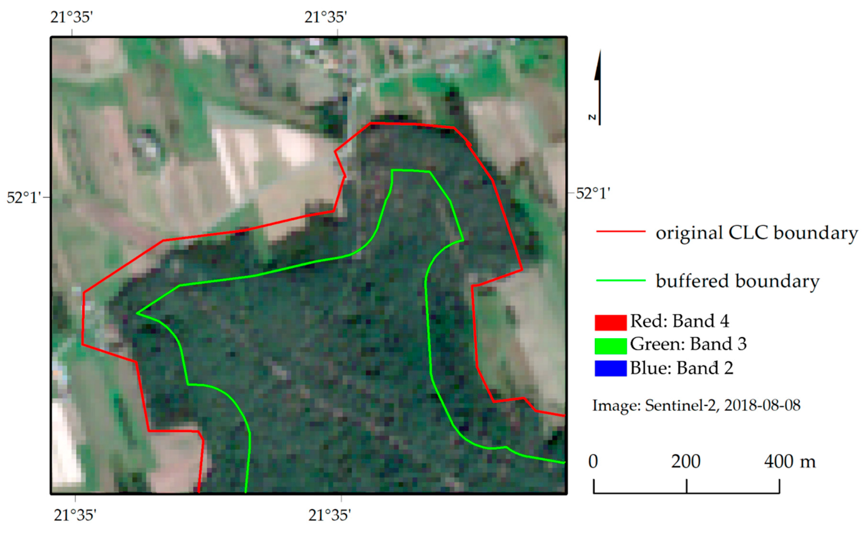The validation of CLC products is a difficult task due to the wide range of distinguished areas that are complex in structure and spectrally heterogeneous, which forces the use of time-consuming optimization procedures [13], e.g., setting the threshold for the maximum number of pixels per class, additionally assigned to the training and test set using a specific sampling method [11]. Besides, to make the reference data representative and reliable, they are reduced by an internal buffer of a specific size, aimed at removing mixed pixels at the edges of the reference polygons [14].

The Landsat and Copernicus missions have gained tremendous popularity in land cover research due to their open access policy [15]. It is often necessary to increase the informational function of acquired images through data fusion. One of the methods used is multi-temporal composition, combining scenes acquired at different dates for the same location [16]. It is based on differences in the spectral reflection of objects depending on the season. This is one of the most commonly used techniques that allow a statistically significant increase in classification accuracy [17]. Gounaridis et al. [18] used such an approach to classify CLC 2012 data where 12 out of 15 Corine classes were identified in the research area, and then a 50 m wide internal buffer was used on the field data representing them. During training, 1000 pixels were chosen randomly for each class, and then the Random Forest algorithm classified the composition of W multi-temporal images obtained by the Landsat Thematic Mapper (TM) and Enhanced Thematic Mapper Plus (ETM+) scanners. An overall accuracy of 83% was obtained. Another possible method is to include vegetation indicators [19].

Altitude data also supplement multispectral data. Leinenkugel et al. [11] used a multi-temporal composition obtained by Enhanced Thematic Mapper Plus (Landsat 7 ETM+) and Operational Land Imager (Landsat 8 OLI) scanners and additionally included the altitude data of the Shuttle Radar Topography Mission (SRTM). Analyses were conducted of three research areas in Europe that are geographically diverse from each other. CLC 2012 served as reference data for land cover, which was prepared by removing mixed pixels using two internal buffers (50 and 100 m wide) to check the effect of their size on classification accuracy. In the research areas, there were 20,000 to 50,000 training pixels for the entire dataset. Classifying with the Random Forest algorithm, overall accuracy was obtained in the range of 55% to 67%, depending on the area. The differences in the classification accuracy between the data on which the 50 and 100 m buffers were used turned out to be small, as the total accuracy values fluctuated by only 1 percentage point in favor of both the data with the larger and smaller buffer.

Multispectral and radar data are also used for research and are combined with digital terrain models. Balzter et al. [14] combined radar data acquired by the Sentinel-1A satellite with SRTM data. Using CLC 2006, a hybrid model was created containing 27 classes [14]. Training and verification pixels were selected at random. Besides, a maximum pixel threshold of 20,000 pixels per class was set, and then, the classification was carried out using the Random Forest algorithm, achieving an overall accuracy of 68%.

Despite the high popularity of multispectral and radar data in land cover studies, Novillo et al. [20] used data collected by the Multiangle Imaging SpectroRadiometer (MISR) located on the Terra platform in order to gather image data for the same area at different sensor inclination angles. Based on 2006 CLC data for level 3, 35 classes were identified, followed by an internal buffer width of 137.5 m. The classification was performed 100 times with the k-means algorithm for each of the seven sensor deflection combinations. The combination with all mirror tilting configurations achieved the highest overall accuracy (70%). The best total accuracy (over 75%) was obtained for the following classes: non-irrigated arable land (211), agro-forestry areas (244), and coniferous forest (312). Many classes obtained poor results (about 20%): construction sites (133), green urban areas (141), fruit trees and berry plantations (222), annual crops associated with permanent crops (241), bare rocks (332), sparsely vegetated areas (333), and inland marshes (411); however, these classes had a small set of samples for training and verification (several dozen pixels).

During the past two decades, the Random Forest (RF) and Support Vector Machine (SVM) classifiers have drawn attention to image classification in remote sensing applications. Sheykhmousa et al. [21] highlighted that in particular, land use and land cover (LULC) mapping is the most common application of remote sensing data for a variety of environmental studies, and based on an extensive review of existing articles, they consider that the growing applications of LULC mapping alongside the need for updating the existing maps have offered new opportunities to effectively develop innovative RS image classification techniques in various land management domains to address local, regional, and global challenges. As a result of the review article, the relatively high similar SVM and RF performance in terms of classification accuracy makes them among the most popular machine learning classifiers within the RS community and demonstrates competitive results with CNNs [21].

Since the Random Forest algorithm is popular in land cover classification and gives satisfactory results, Rodriguez-Galiano et al. [22] conducted a detailed analysis of the impact of input data properties on classification accuracy. On the multi-temporal composition of images obtained by the TM scanner, they determined 14 land cover classes. They checked the impact of data reduction on the overall accuracy of the classification. On the one hand, it saves time in the classification process, and on the other hand, it is necessary to have a representative number of samples for each class. It was found that only when the training dataset was reduced by 70%, overall accuracy decreased. They used the same methodology when checking the classifier’s resistance to the influence of noisy data, which can often negatively affect the accuracy of the classification, e.g., using 50% of the noisy data, the out-of-bag (OOB) error increased significantly [23].

Although there are many studies on land cover classification [24] in the literature, few studies address the Corine Land Cover classification, specifically, level 3. The class definition characteristics of the Corine Land Cover make the land cover types included in the project only present in Europe, so it is not easy to compare it with classifications made for other areas, which narrows the scope of comparison. Current Corine Land Cover classification studies mostly cover small areas and referred to the generalized first and second levels [25]. Corine Land Cover has numerous limitations [26], and the new edition of CLC+ is intended to overcome them. One of its elements will be pixel-based classification, which makes it necessary to check the classification’s accuracy for particular classes. The results obtained in the study may provide valuable information for the teams preparing classifications for individual European areas. The main source of optical data in the CLC+ project is the multi-temporal data acquired by the Sentinel-2 satellite, with the Landsat 8 satellite filling in any gaps in the data; therefore, in this paper, data acquired by both Sentinel-2 and Landsat 8 satellites were checked to show the classification accuracy discrepancies depending on data types.

Additionally, by comparing the most popular machine learning algorithms such as Random Forest and Support Vector Machines, the bias of classifications that are often based on a single method was reduced. Due to the ease of implementation of the algorithms used, it is possible to reproduce the results and make them comparable easily. The influence of the number of pixels per class to achieve a given overall accuracy was also examined in this study. This helps determine the number of samples required when collecting master data and preparing it for classification in a CLC project. This study was undertaken due to the lack of comparative studies in the literature on CLC classes over varying areas, comparing classifiers and using iterative accuracy assessment.

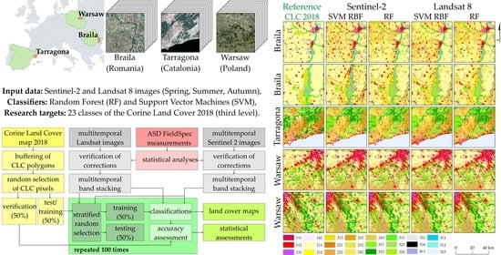
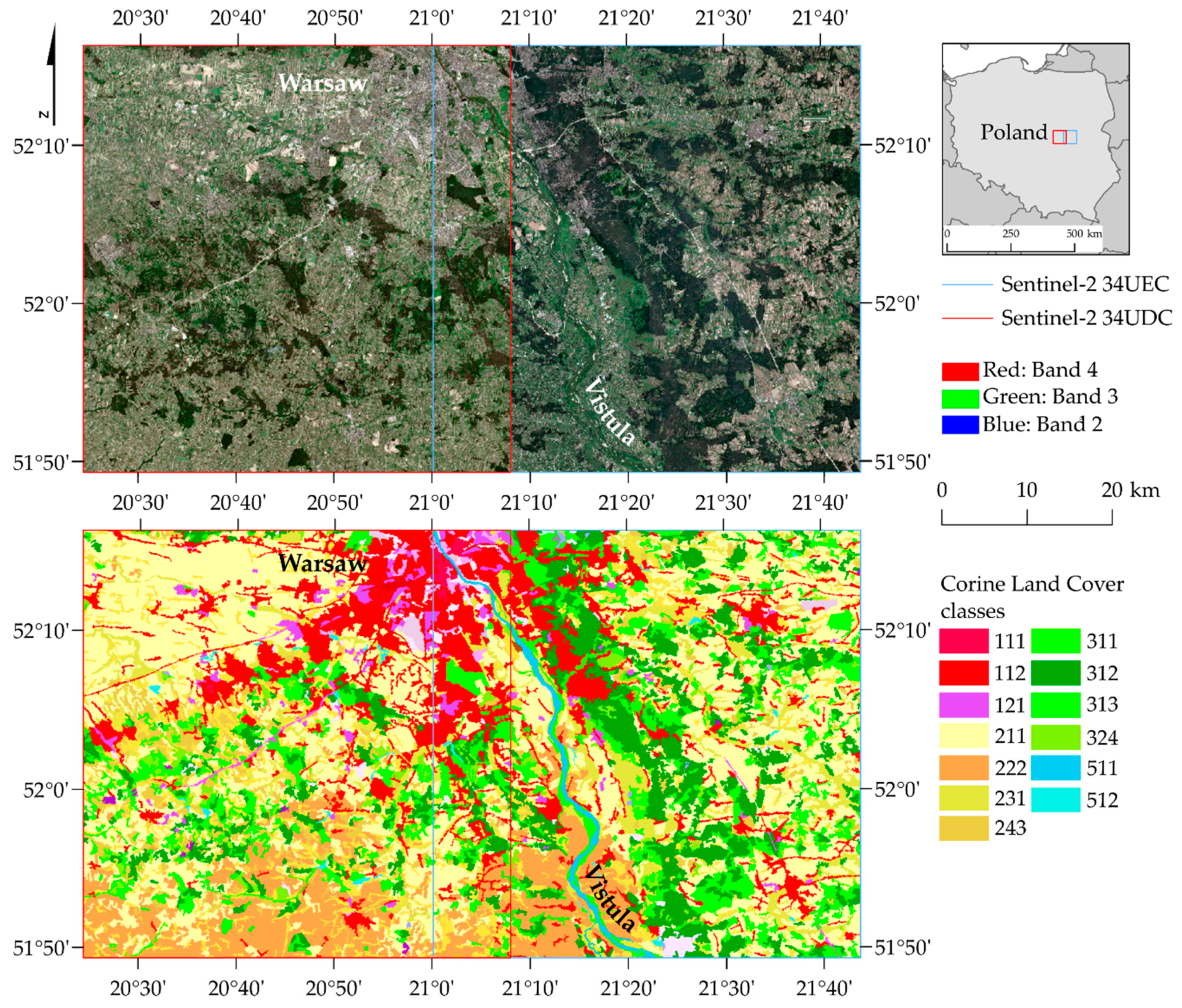
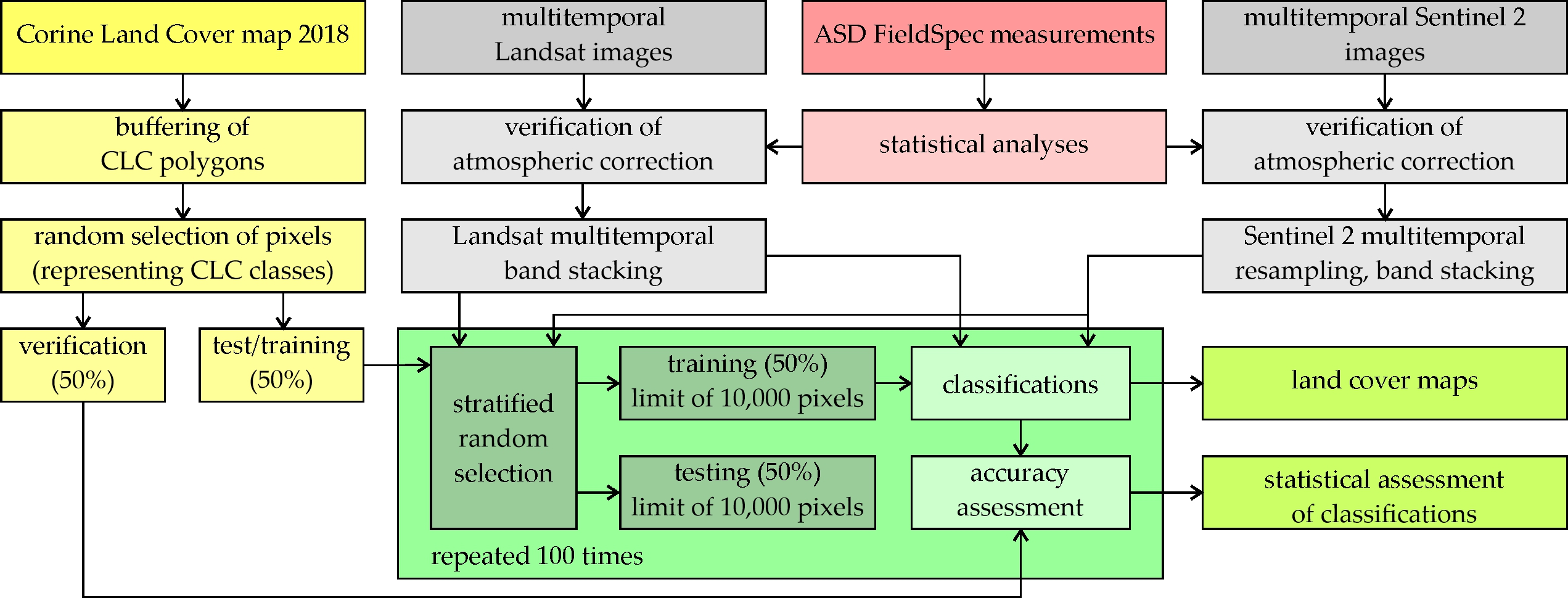
Our intention in this study was to assess the automatic land classification accuracy according to Corine guidelines based on Sentinel-2 and Landsat 8 multitemporal images (spring, summer, and autumn 2018/2019). For this purpose, areas located in various European Union parts, with a diversified history, spatial management, land cover, and different cartographic traditions were selected; however, due to the Corine program guidelines, the minimal mapping unit had to be 500 × 500 m, which significantly reduced the image information potential. The research procedure was based on two scenarios: 1) classification of twenty-meter pixel classification of the Sentinel-2 bands (10 m pixels were resampled to 20 m) and also on the thirty-meter pixel sizes of the Landsat 8; 2) in the next step, all pixels were resampled to 60 m, the basic classifications were made on them, and the results were generalized with a majority filter to the size of 8 × 8 pixels (480 × 480 m compared to the required 500 × 500 m in the Corine program). This allowed us to assess the effectiveness of the classifiers and allowed for the potential of automatic classification according to the official European CLC 2018 dataset. CLC data served as the input layer and were divided into training (25%), test (25%), and validation (50%) sets. Random Forest (RF) and Support Vector Machine (SVM) algorithms in the open-source R programming language were used as the classifiers. The main idea was to verify free-of-charge methods, which can be easily implemented on multicore processors. The classification patterns were randomly selected based on the 3rd CLC level. One of the key elements was the impact of the number of training pixels on the obtained results; it allowed us to optimize field reconnaissance during a verification phase (in the research, we used archival (2018) CLC layer and responsible satellite images).

2. Materials and Methods

Densely populated metropolitan with surrounding suburban areas characterized by very heterogeneous land cover, but also fragments of large-scale farming and protected areas on five research areas were selected, each covering an area of 50 × 50 km, located in Romania (northern and southern Braila), Catalonia (Tarragona), and in Poland (eastern and western part of Warsaw). This enabled diverse land cover forms to test the impact of geographic variability as well as local variations resulting from the Corine Land Cover national teams. In each country, the areas depicted on the cloudless Sentinel-2 granules as well as on the Landsat 8 image fragment were selected. Multispectral image data were acquired in spring, summer, and autumn 2018, but due to intense cloud cover on some of the collected scenes, the decision was made to replace them with data acquired in 2019.

2.1. Research Areas

Braila (Romania) is a 4700 km² county situated in eastern Romania. Braila is a medium-size county representing 2% of the total area of Romania (Figure 1). The main geographic characteristic is the Baraganului Plain because it is surrounded in the Eastside by the Danube river. The surface is flat and crossed by Buzau, Calmatui, and Siret river confluences. Here, the Danube forms an island called The Big Island of Braila with a surface of 710 km², used mainly in agriculture, and a group of seven small islands with dominant swamps called The Small Island of Braila and contains the Natural Park Small Pound of Braila. Braila is known as an agricultural county because of the soil quality, mostly chernozem, resulting in 80% of the entire county surface (except urban areas) being used as arable land. The main crops cultivated in the area are grain, corn, barley, oats, sunflower, soy, and rye [27,28]. The urban centers are the cities of Braila and Galati, including the Braila district and fragments of four other districts.

The Tarragona (Catalonia) research area (Figure 2) is located in Tarragona’s province on the Mediterranean Sea coast, along the famous tourist region of Costa Dorada. The designated area includes the Prades mountain range with oak and pine forests. The area is characterized by rich topography with height differences up to 1203 m a.s.l. (Tossal de la Baltasana). Agriculture consists mainly of vineyards, olive groves, and hazelnut cultivation [29]. The main type of soil is calcareous soil, as well as regosol and lessive soil. The river network is poorly developed, there are also no water reservoirs. The largest city in the region is Tarragona, an important center of the petrochemical industry that exerts a strong anthropopressure on the environment by emitting large amounts of air pollutants [30].

The Warsaw (Poland) area includes a fragment of the Mazovian Lowland (Masovian Plain), the largest geographical region in central Poland; see Figure 3. The river network consists of the Vistula and its tributaries, the Wieprz and Pilica, and the Sulejowski reservoir is a characteristic hydrological object. The distribution of soils is characterized by considerable diversification, mainly light soils (arenosols and podzolic), as well as lesser soils and marshes in the river valleys and floodplain terraces. Most of them are not very fertile. The species structure of forest communities consists mainly of pine forests with an admixture of birch, oak, and alder. Agricultural land is predominant, and south of Warsaw is one of Poland’s largest orchard areas [31]. The main urban center in the region is Warsaw, which is densely built and populated, resulting in a strong anthropopressure on the environment through significant emissions of air pollutants [32], and the transformation of the landscape through intensive urbanization [33].

2.2. Methods

The effectiveness of satellite image classifications according to the Corine Land Cover guidelines was evaluated according to the following methods (Figure 4):

• Sentinel-2 and Landsat 8 satellite image acquisition. The images were acquired, then the accuracy of atmospheric and geometric corrections was assessed (by identifying pixels with ground patterns for atmospheric correction, and then verification by overlapping multitemporal images, despite the acquisition of data for the same scene, the pixels of individual images may differ. For this purpose, the pixel grids of the images were harmonized and aligned),
• obtaining official Corine Land Cover data for 2018 from the European Environment Agency (EEA),
• assigning a common frame with satellite images by polygon buffers to eliminate pixels of surrounding land cover forms,
• the random selection of pixels represents different land cover forms,
• optimization of SVM and RF classifiers, iterative accuracy assessment (100 times),
• image classifications with the best algorithms and parameters, accuracy assessment,
• final review of land cover maps.

2.2.1. Input Data

Sentinel-2 images (level 2A) were acquired using Copernicus Open Access Hub. Only scenes with cloudiness not exceeding 10% were selected for further processing (

Table 2. Used satellite images (*—2019).

Satellite	Orbit	Spring 2018	Summer 2018	Autumn 2018
Sentinel-2	34UDC (Poland)	08 April	07 June	20 September
	34UEC (Poland)	10 April	08 August	06 November
	34TNL/34TNK (Romania)	26 April	14 August	31 October
	31TCF Catalonia	18 April	10 August	24 November
Landsat 8	187/24 (Poland)	08 April	30 August	01 October
	188/24 (Poland)	02 April *	24 August *	27 October *
	181/29 (Romania)	30 April	23 August	14 October
	182/28, 182/29 (Romania)	23 May	14 August *	01 October *
	198/31 Catalonia	21 April	26 July	28 September

). First, in the ENVI 5.3 software, all bands were resampled to the pixel size of sixty meters using the nearest neighbor method. For each research area, multitemporal compositions were created, collecting the spring, summer, and autumn scenes. The images were exported to the GeoTIFF format. Landsat 8 data were collected based on the Earth Resources Observation and Science (EROS) Science Processing Architecture (ESPA) service, in which images were ordered with surface reflectance already performed. In the ENVI 5.3 program, the same procedures of resampling to 60 m pixel size, layer stacking, and exporting to GeoTIFF were carried out.

The acquired Sentinel-2 and Landsat 8 images were corrected atmospherically; Sentinel-2 atmospheric correction was based on an algorithm proposed in Atmospheric/Topographic Correction for Satellite Imagery [34]. The method performs atmospheric correction based on the LIBRADTRAN radiative transfer model [35]. Landsat 8 applies Land Surface Reflectance Code (LaSRC), based on the 6S radiative transfer model and a heritage from the MODIS MCD09 products [36]. Nevertheless, due to the analysis of images from different periods and areas, the authors verified the atmospheric correction quality. For this purpose, a ground-based ASD FieldSpec 4 (with the ASD ContactProbe; Analytical Spectral Devices, Inc., Longmont, CO, USA) spectrometric measurements of large 59 homogeneous and dominant calibration targets (asphalt, concrete, gravel, and paving stones) in Warsaw and surrounding areas were made. In the first step, the ASD FieldSpec spectrometric data were resampled to the resolution of Sentinel-2 and Landsat OLI, and then, pixel values corresponding to the localization of the field polygons on which the ground measurements were collected. The comparison results are the values of the Root Mean Square Error (RMSE); the results are presented in the Appendix A,

Table A1. Root mean square errors (RMSE) between ground calibration targets and atmospherically verified used Sentinel-2 and Landsat images (Warsaw research targets).

Polygon		Sentinel-2 (34 EUC)			Sentinel-2 (34 EDC)			Average	Landsat 8			Average
		10 April	8 August	6 November	8 April	7 June	20 September		8 April	30 August	1 October
asphalt	w12	0.05	0.07	0.04	-	-	-	0.06	0.09	0.08	0.07	0.08
	w14	0.03	0.06	0.05	-	-	-	0.05	0.05	0.08	0.09	0.07
	w17	0.02	0.04	0.02	-	-	-	0.03	0.02	0.03	0.04	0.03
	w18	0.03	0.05	0.06	-	-	-	0.05	0.07	0.09	0.09	0.08
	w19	0.03	0.05	0.06	-	-	-	0.04	0.07	0.07	0.08	0.08
	w20	0.03	0.05	0.05	-	-	-	0.04	0.05	0.08	0.08	0.07
	w23	0.03	0.04	0.06	-	-	-	0.04	0.03	0.04	0.03	0.03
	w25	0.02	0.04	0.05	-	-	-	0.03	0.02	0.04	0.03	0.03
	w28	0.06	0.08	0.06	-	-	-	0.06	0.03	0.06	0.06	0.05
	w31	0.06	0.06	0.02	-	-	-	0.05	0.06	0.07	0.06	0.06
	w32	-	-	-	0.03	0.09	0.07	0.06	-	-	-	-
	w34	-	-	-	0.08	0.13	0.11	0.11	-	-	-	-
	w37	-	-	-	0.04	0.09	0.08	0.07	-	-	-	-
	w40	0.05	0.09	0.06	0.04	0.09	0.06	0.06	0.03	0.08	0.09	0.07
	w43	0.04	0.06	0.02	0.03	0.08	0.04	0.05	0.03	0.05	0.05	0.04
	w49	0.03	0.06	0.04	0.02	0.05	0.05	0.04	0.03	0.04	0.03	0.03
	w51	0.04	0.05	0.05	0.02	0.04	0.04	0.04	0.02	0.03	0.02	0.02
	w54	0.04	0.05	0.03	0.03	0.04	0.04	0.04	0.03	0.04	0.03	0.03
	w55	0.03	0.06	0.06	0.03	0.05	0.04	0.05	0.06	0.08	0.08	0.07
	w57	0.03	0.06	0.03	0.02	0.06	0.04	0.04	0.03	0.05	0.03	0.03
	w60	0.03	0.06	0.05	0.04	0.07	0.05	0.05	0.04	0.05	0.05	0.05
	w61	0.06	0.12	0.05	0.06	0.11	0.09	0.08	0.06	0.08	0.07	0.07
	w63	0.05	0.07	0.07	0.07	0.05	0.06	0.06	0.08	0.09	0.10	0.09
	w8	0.03	0.04	0.03	-	-	-	0.03	0.04	0.05	0.06	0.05
gravel	w33	-	-	-	0.05	0.04	0.05	0.05	-	-	-	-
	w38	0.08	0.09	0.12	0.12	0.10	0.09	0.10	0.14	0.15	0.15	0.15
	w39	0.06	0.07	0.13	0.06	0.08	0.08	0.08	0.10	0.17	0.18	0.15
	w48	0.12	0.10	0.20	0.14	0.10	0.12	0.13	0.14	0.15	0.15	0.14
	w58	0.05	0.07	0.08	0.06	0.07	0.07	0.07	0.08	0.09	0.09	0.09
	w62	0.03	0.07	0.03	0.02	0.08	0.07	0.05	0.02	0.07	0.06	0.05
concrete pavement	w11	0.02	0.06	0.04	-	-	-	0.04	0.03	0.05	0.04	0.04
	w13	0.05	0.07	0.04	-	-	-	0.05	0.04	0.05	0.05	0.05
	w16	0.02	0.03	0.05	-	-	-	0.03	0.04	0.05	0.06	0.05
	w21	0.04	0.08	0.03	-	-	-	0.05	0.04	0.07	0.08	0.06
	w26	0.02	0.05	0.04	-	-	-	0.04	0.03	0.05	0.04	0.04
	w27	0.02	0.04	0.04	-	-	-	0.04	0.06	0.07	0.08	0.07
	w30	0.05	0.04	0.11	-	-	-	0.07	0.05	0.07	0.07	0.07
	w35	-	-	-	0.03	0.05	0.03	0.04	-	-	-	-
	w36	-	-	-	0.02	0.07	0.05	0.05	-	-	-	-
	w41	0.05	0.11	0.06	0.04	0.12	0.09	0.08	0.05	0.10	0.11	0.08
	w42	0.02	0.04	0.06	0.04	0.04	0.04	0.04	0.04	0.07	0.09	0.07
	w44	0.04	0.07	0.06	0.04	0.08	0.04	0.05	0.04	0.06	0.06	0.05
	w45	0.03	0.03	0.04	0.05	0.03	0.03	0.04	0.06	0.08	0.08	0.08
	w50	0.02	0.02	0.07	0.04	0.03	0.03	0.03	0.05	0.05	0.06	0.05
	w52	0.03	0.05	0.04	0.02	0.04	0.04	0.04	0.02	0.03	0.03	0.02
	w53	0.02	0.04	0.08	0.03	0.02	0.03	0.04	0.05	0.06	0.06	0.06
	w56	0.07	0.06	0.11	0.08	0.08	0.08	0.08	0.11	0.12	0.13	0.12
	w59	0.03	0.05	0.04	0.03	0.06	0.06	0.05	0.03	0.05	0.05	0.04
	w10	0.03	0.10	0.03	-	-	-	0.05	0.02	0.05	0.04	0.04
	w15	0.02	0.03	0.04	-	-	-	0.03	0.05	0.05	0.05	0.05
	w22	0.03	0.07	0.04	-	-	-	0.05	0.03	0.06	0.07	0.05
	w24	0.05	0.04	0.10	-	-	-	0.06	0.04	0.04	0.05	0.04
	w29	0.02	0.03	0.02	-	-	-	0.02	0.01	0.04	0.03	0.03
Average		0.04	0.06	0.06	0.05	0.07	0.06	0.05	0.05	0.07	0.07	0.07

.

Corine Land Cover data for 2018 were downloaded as the shapefile using the Copernicus Land Monitoring Service. Corine’s and image data were clipped to specific research areas and projected into Universal Transverse Mercator (UTM) coordinate system (UTM 31N—Catalonia, UTM 34N—Poland, UTM 35N—Romania).

Internal buffer with a width of 100 m was used to minimize the negative edge impact on the spectral land cover patterns by reducing each polygon by its size (Figure 5). The value of the buffer width was selected due to Corine Land Cover’s technical specification, which specified that the drawn boundaries’ geometric accuracy is greater than 100 m [4]. Polygon buffers were automatically created, and the small polygons with an area less than 25 ha were filtered. Due to the errors noticed in the Corine Land Cover 2018 map, a verification by photointerpretation of 2018 Sentinel-2 satellite images was made [37], and the total area used for classification and its proportions between classes for each area vary, indicating an unbalanced dataset (

Table 3. Used areas for testing, training, and validation.

		Warsaw (Poland)		Braila (Romania)		Catalonia
		34UDC	34UEC	35TNL	35TNK	31TCF
Class	Description	Area (ha)	Area (ha)	Area (ha)	Area (ha)	Area (ha)
111	Continuous urban fabric	82.5	63.6	-	-	89.9
112	Discontinuous urban fabric	4369.4	2478.4	4229.9	960.2	323.8
121	Industrial or commercial units	449.2	199.0	790.5	-	416.3
142	Sport and leisure facilities	101.2	65.0	-	-	-
211	Non-irrigated arable land	4383.7	6753.6	5312.8	10,138.5	509.4
212	Permanently irrigated land	-	-	-	-	57.3
213	Rice fields	-	-	411.6	2261.3	-
221	Vineyards	-	-	-	-	882.9
222	Fruit trees and berry plantations	1109.6	2998.4	-	-	140.3
223	Olive groves	-	-	-	-	47.8
231	Pastures	153.9	1213.1	851.0	1022.9	-
242	Complex cultivation patterns	-	-	504.2	634.6	1936.1
243	Land principally occupied by agriculture, with significant areas of natural vegetation	32.0	106.4	165.0	-	-
311	Broad-leaved forest	157.7	496.0	370.2	1583.4	441.6
312	Coniferous forest	307.6	4015.0	-	-	948.9
313	Mixed forest	112.7	635.3	-	-	-
323	Sclerophyllous vegetation	-	-	-	-	-
324	Transitional woodland/shrub	86.4	106.2	46.0	264.4	43.2
331	Beaches, dunes, sands	-	-	-	-	3.3
411	Inland marshes	-	-	225.6	411.5	-
511	Water courses	37.4	147.0	286.3	209.7	-
512	Water bodies	22.9	21.4	1823.0	137.9	-
523	Sea and ocean	-	-	-	-	49,303.5

); therefore, each dataset was balanced with a threshold of 100, 200, 300, 400, and 500 pixels. For machine learning algorithms, it is important to balance the dataset. The main reason for this is to give equal priority to each class during the training process.

2.2.2. Classification and Accuracy Assessment

The procedures presented in this section were conducted using the R programming language and the R Studio 4.0.0 integrated development environment [38,39,40]. The first step was to extract each class’s patterns from the image pixels using the raster and rgdal packages [41,42]. Then, on the obtained datasets, the algorithm training parameters were optimized, and the tuning of all classifiers’ parameters was performed on its entire set of patterns. The parameter optimization procedures were performed on the references derived from the Multispectral Instrument Sentinel-2 (MSI) and Landsat 8 OLI images (

Table 4. Optimized parameters of the classifiers.

Classifier	Hyperparameters	Sentinel-2 (60 m)	Landsat 8 (60 m)
RF	ntree	500	500
	mtry	13	10
SVM linear	cost	100	100
SVM RBF	cost	10	1
	gamma	0.1	0.01
SVM polynomial	cost	100	1
	gamma	0.1	0.01
	coef0	0	0
	degree	3	3
SVM sigmoid	cost	100	1
	gamma	0.1	0.01
	coef0	0	0

). The randomForest package was used to implement the Random Forest algorithm [43]. The ntree parameter was set to 500 because the OOB error values above this number usually stabilize [44]. Tuning was applied to the mtry parameter, and the mtry with the lowest OOB error value was selected. In the case of the Support Vector Machines algorithm, the e1071 package was used as an implementation [45]. The learning parameters were optimized using the grid search method, where each combination of the parameters is checked from the pool of parameters. Tuning was performed for linear, polynomial, radial kernel function (RBF), and sigmoid kernel functions. The coef0 parameter for polynomial and sigmoid kernels was left at the default value of 0 and the degree parameter for the polynomial kernel was left at its default of 3.

One of our goals in this study was to compare the accuracy of classification according to algorithms and the number of pixels used in training. Scenarios were prepared to focus on an influence of 100, 200, 300, 400, and 500 pixels for each class of the training set. For this purpose, an iterative accuracy assessment was used, which was repeated 100 times, according to the following steps

• random selection of reference pixels for training and testing datasets in the 50:50 ratio, it was ensured that they were divided according to their belonging to a polygon (pixels from a given polygon could be included in only one of the datasets (training or test) in order to meet the condition of their independence [37]. The rngtools and doRNG packages were used to generate random seeds and optimize the iterative accuracy assessment’s execution time. The multiple cores of the processor utilized doParallel, and foreach package using a PSOCK (Parallel Socket Cluster), a cluster was used [46,47].
• resampling of a proper number of pixels for training (previous step),
• training of Random Forest and Support Vector Machines classifiers,
• accuracy assessment of each classification,
• saving classification accuracy results and a random seed.

Then, the classification accuracy of the remaining areas was assessed on the algorithms’ selected parameters, where the parameters turned out to be satisfactory in all cases. The following metrics were used to assess the classification accuracies [48]:

• overall accuracy (OA)—the ratio of all correctly classified pixels to the sum of all pixels,
• producer accuracy (PA)—the ratio of correctly classified pixels of a given class to all reference pixels of a given class,
• user accuracy (UA)—the ratio of correctly classified pixels of a given class to all pixels classified to this class,
• Kappa coefficient measures the correspondence between two datasets, each of which identifies items into mutually exclusive categories presenting how much better the classifier is performing over the performance of a classifier that simply guesses at random according to the frequency of each class. Kappa is always less than or equal to 1. Values of 0 or less indicate that the classifier is useless. There is no standardized way to interpret its values. Kappa coefficient was used only to present the final results, but the index is characterized by a high correlation with the overall accuracy, and thus the redundancy of information is doubled [49,50].
• F1-score—is the weighted harmonic mean of the user and producer accuracy [51].

A confusion matrix was also used, which presented correctly classified pixels in its diagonal [48]. Box plots were also used (Figure 6).

Then, the average accuracy of all classes’ F1-score coefficient values was compared in the acquired results. The best algorithms were selected to test the effect of the number of training pixels on the classification accuracy (five classification scenarios were verified in which 100, 200, 300, 400, and 500 pixels were tested per class in the training and testing sets, as well).

For the final maps’ production, models with the highest average F1-score for all scenario classes were selected. Finally, according to the Corine guidelines, a median filter with an 8 × 8 window was used (it means that pixel size is 60 m, so areas smaller than 480 × 480 m were excluded, confirming the CLC rules to eliminate smaller areas than 500 × 500 m, which is the Minimum Mapping Unit of the Corine program). The land cover classes of the final results were colored following the Corine Land Cover specification [4].

3. Results

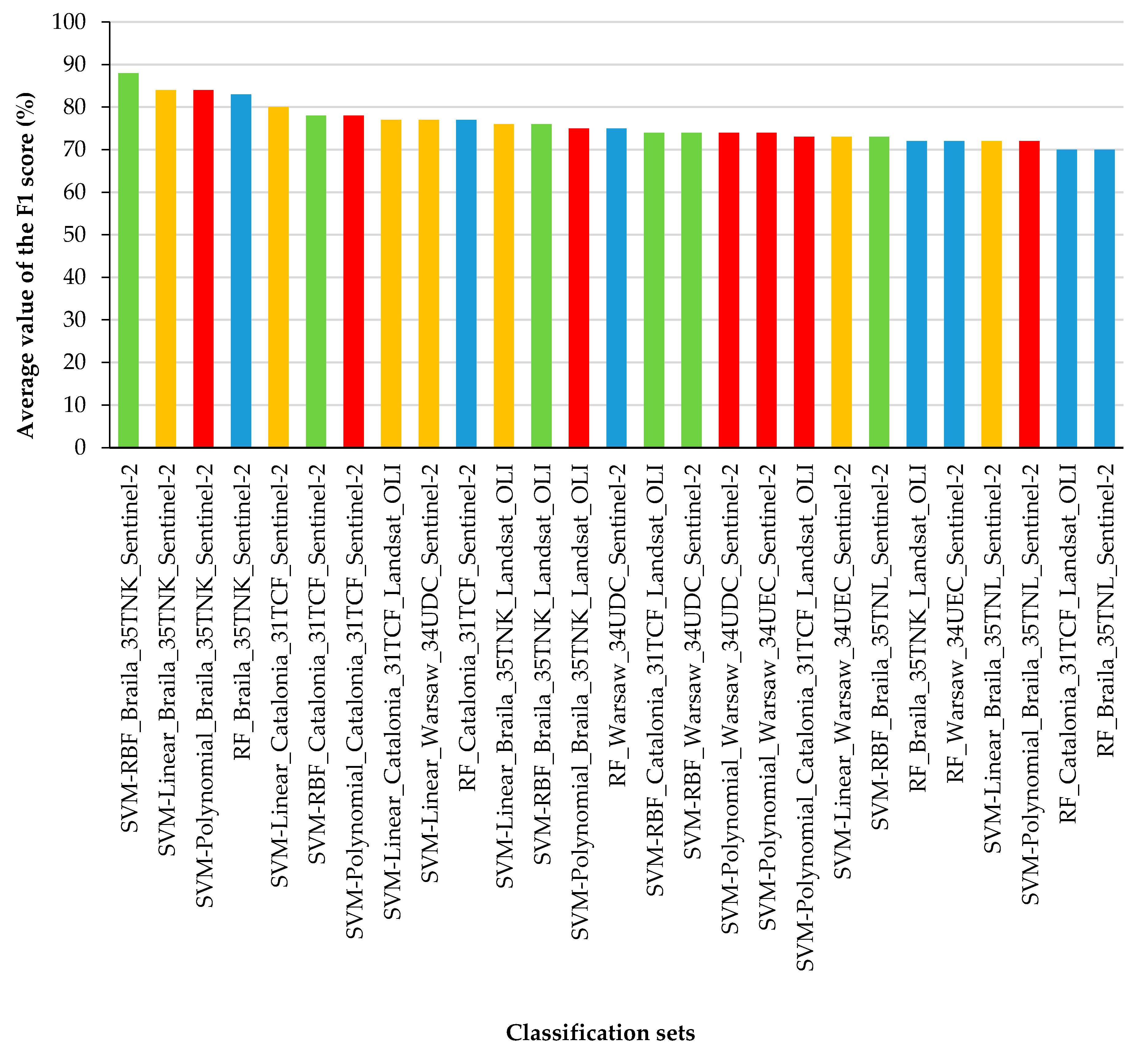
Evaluation of individual classifiers and datasets, their results for the average F1-score of all classes need to be compared (Figure 7). Sentinel-2 images scored the top seven, while the SVM classifiers took the top three best places (RBF, linear, and polynomial kernel functions). Large and homogeneous southern Braila polygons (35TNK) scored the top four on the Sentinel-2 data (F1-score achieved 88%). In the case of images obtained by the Landsat OLI sensor, the best classifier was the SVM algorithm with a linear kernel function for the Catalonia area (F1-score oscillated around 77%). The worst results were obtained for the Random Forest classifier for the Landsat 8 satellite for Catalonia (70% F1) and Sentinel-2 for northern Braila (70% F1).

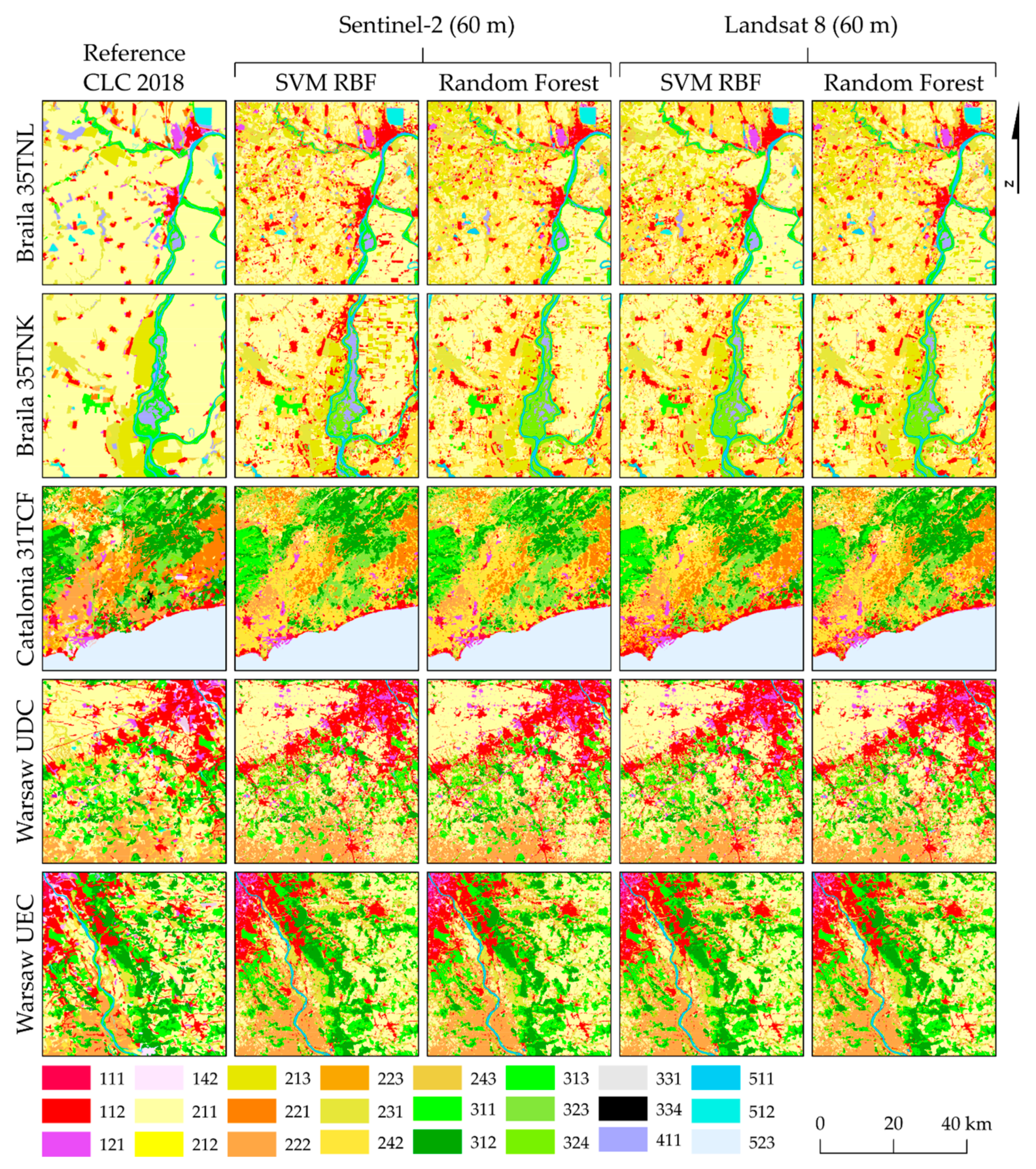
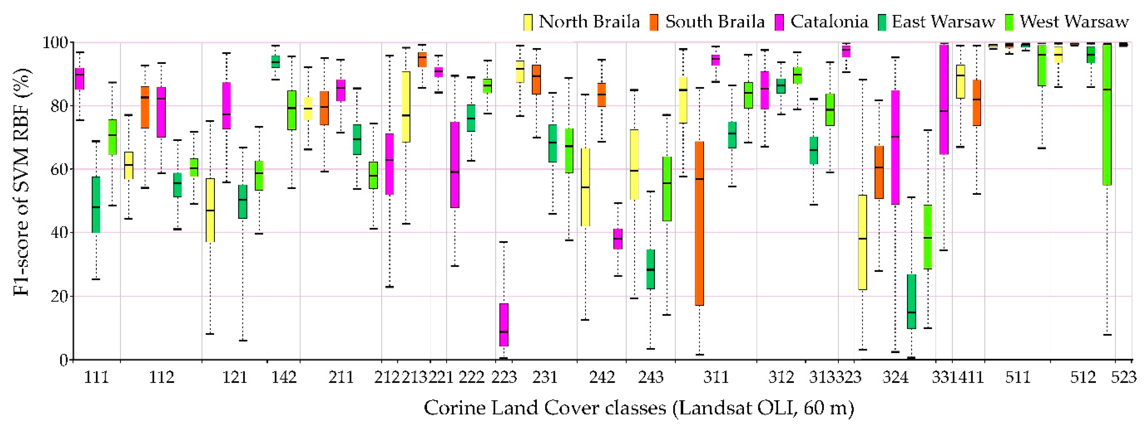
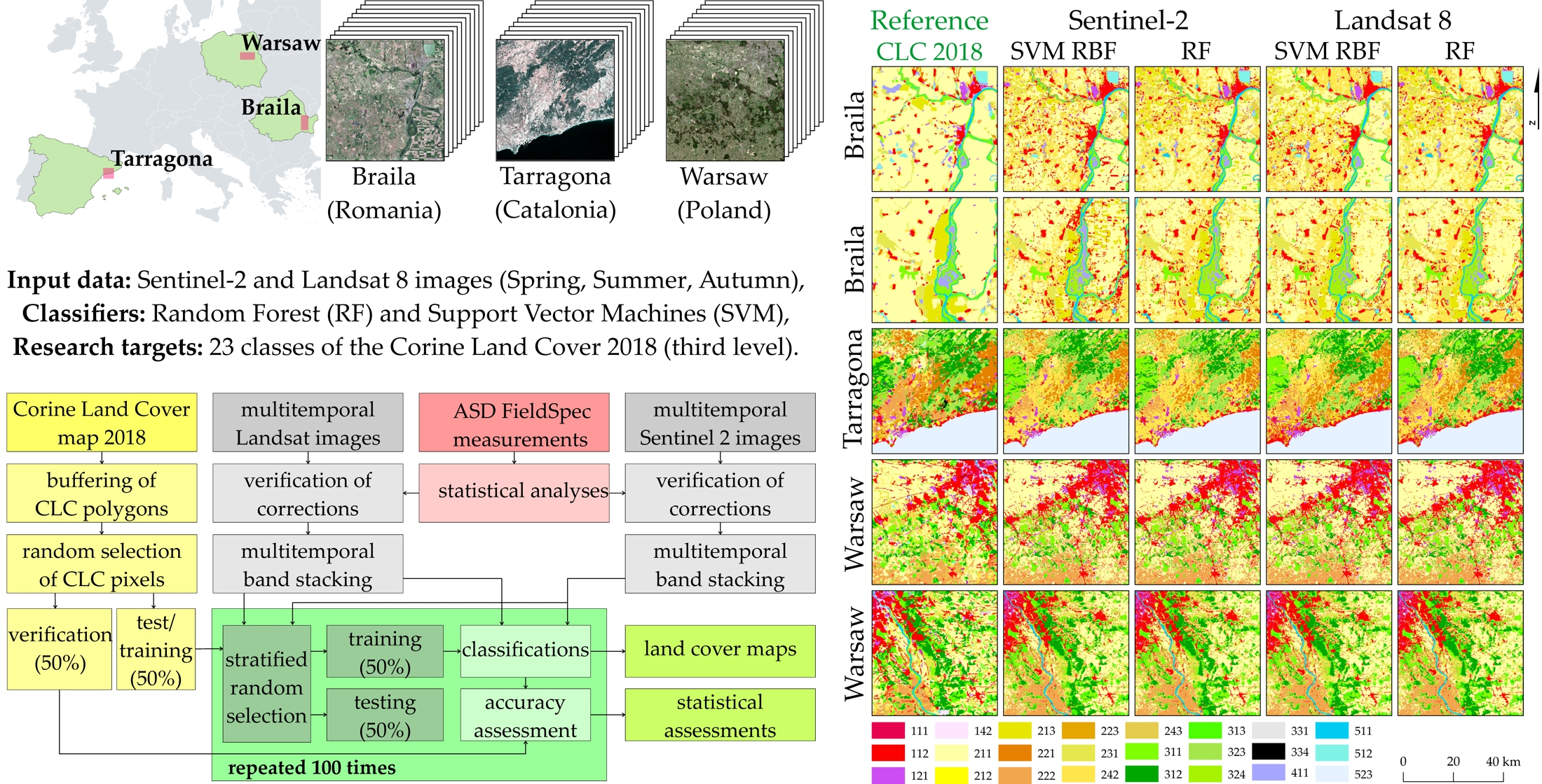
The Support Vector Machine algorithm with the radial kernel function (SVM RBF) algorithm achieved very good results for all areas and all classes of the research (the highest average accuracies of the F1-score oscillating between 73% and 88%; Figure 8); therefore, the further focus was on this classifier and on the Random Forest (it achieved up to 5% lower results than SVM RBF), predicting the result images on both the Sentinel-2 and Landsat 8 imagery. Comparing the classification outcomes with the original Corine Land Cover maps, it can be seen that post-classification maps contain more details, which can be seen in particular in more heterogeneous areas. There is also a difference in the degree of generalization between the Landsat 8 and Sentinel-2 images, which show land cover in more detail. In terms of classifiers, the difference is particularly noticeable for the areas of Braila, where the Random Forest classifier generalized agricultural areas more than the Support Vector Machine, which classified technical objects and roads as class 112 (discontinuous urban fabric). For research areas in Romania, there are significant differences in the case of class 242 (complex cultivation patterns), which in the original study was strongly underestimated comparing with class 211 (non-irrigated arable land). As for the area of northern Braila, there is a discrepancy in the identification of water reservoirs (class 512), which remained without water on the satellite images during the analyzed period. In the case of Catalonia, in relation to the original Corine Land Cover map, there was a change of classes 221 (vineyards) and 222 (fruit trees and berry plantations), which should be identified as class 242 (complex cultivation patterns). Particular differences in the classification of the above-mentioned classes can be noticed between the Sentinel-2 and Landsat 8 images. There are visible differences in the distinction between forest types, e.g., coniferous forests (312), which have decreased compared to deciduous forests (311). In the Catalonia area, the building classes were very well distinguished: 111 (continuous urban fabric), 112 (discontinuous urban fabric), and 121 (industrial or commercial units). In the case of Warsaw granules, fruit trees and berry plantations were classified well (222). As in Catalonia, the different forest classes (311, 312, and 313) were distinguished in more detail than in the original CLC study. The Sentinel-2 images show the Fruit trees and berry plantations class (222) in more detail than the Landsat images. Difficulties were noticed in distinguishing classes 111 (continuous urban fabric) and 121 (industrial or commercial units) due to mixed pixels representing different classes characterized by granularity, discontinuity, and mosaic character (Figure 8).

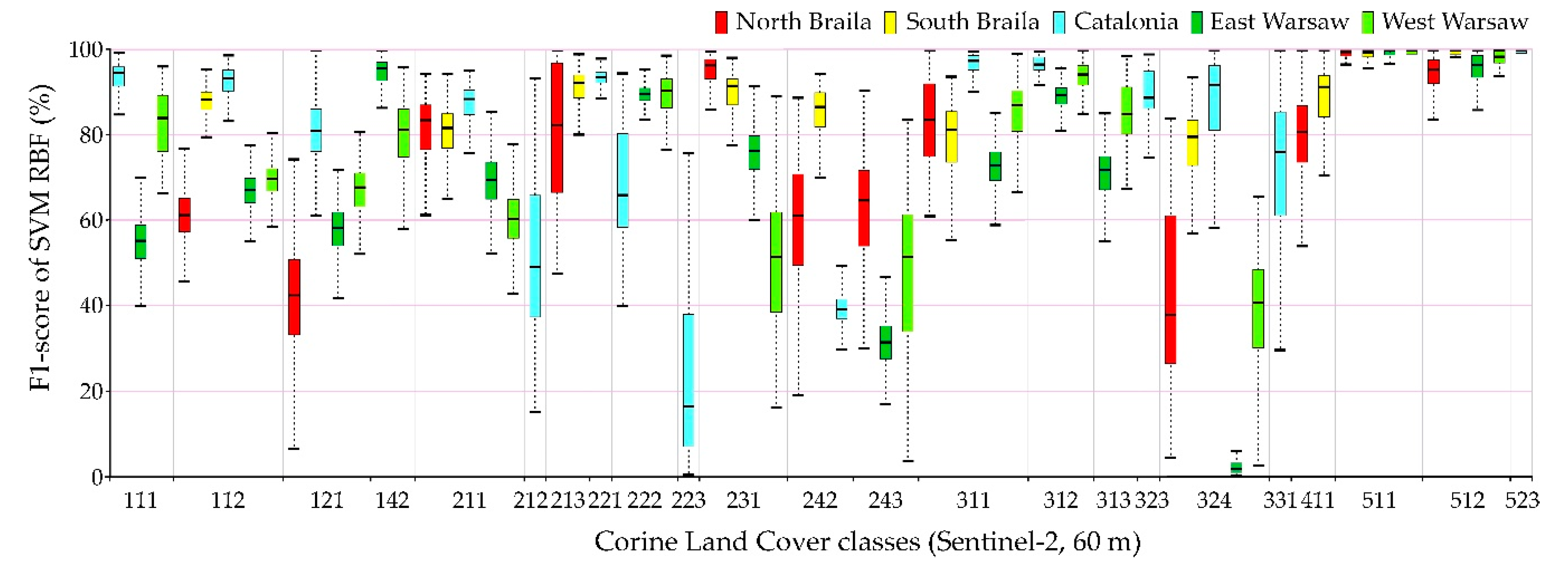
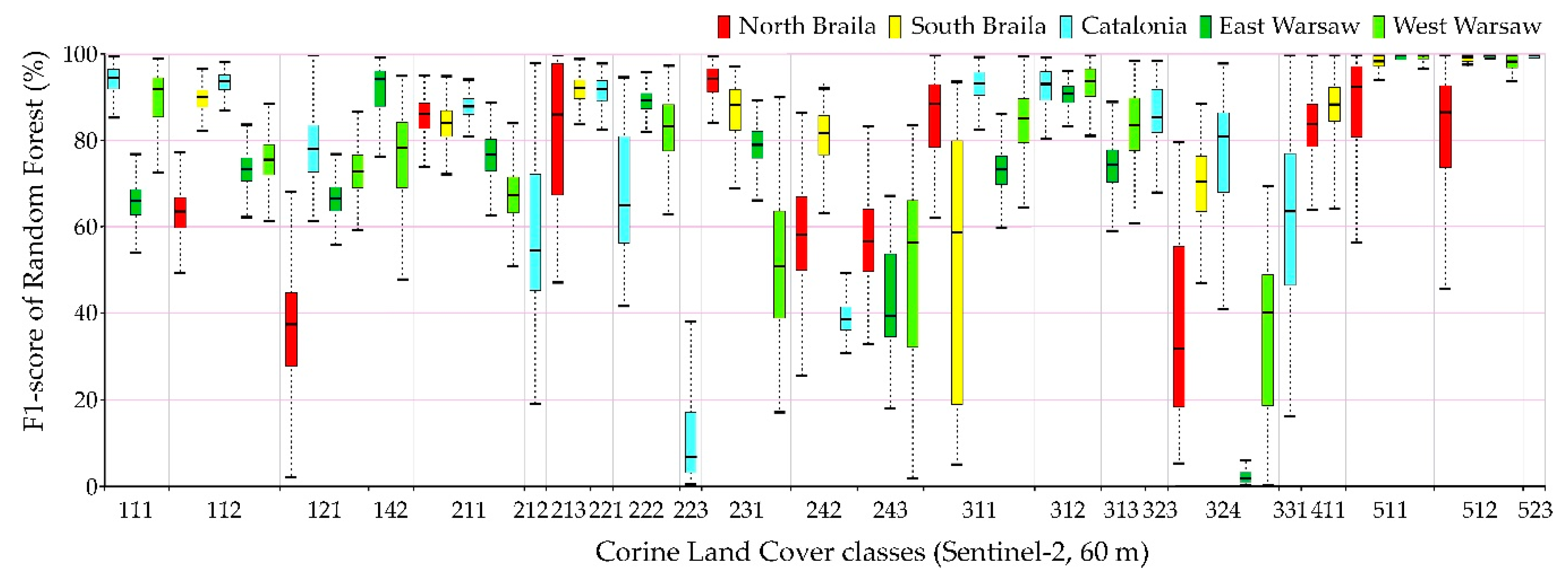
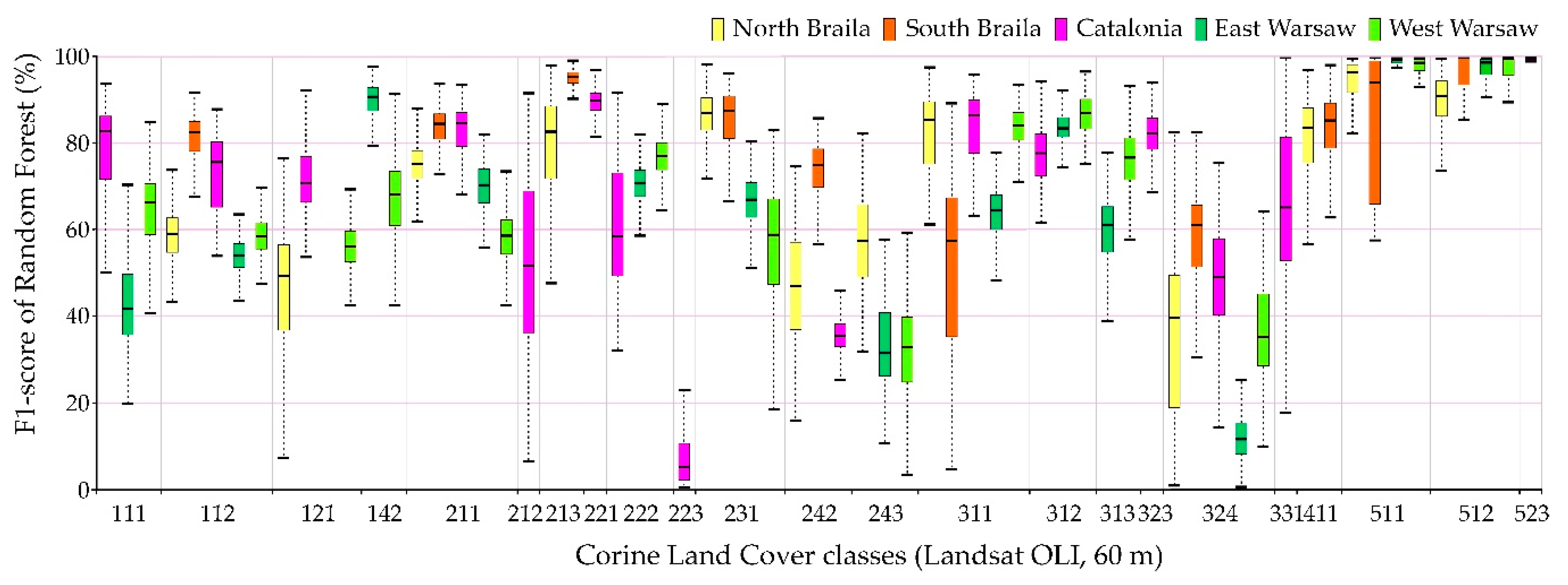
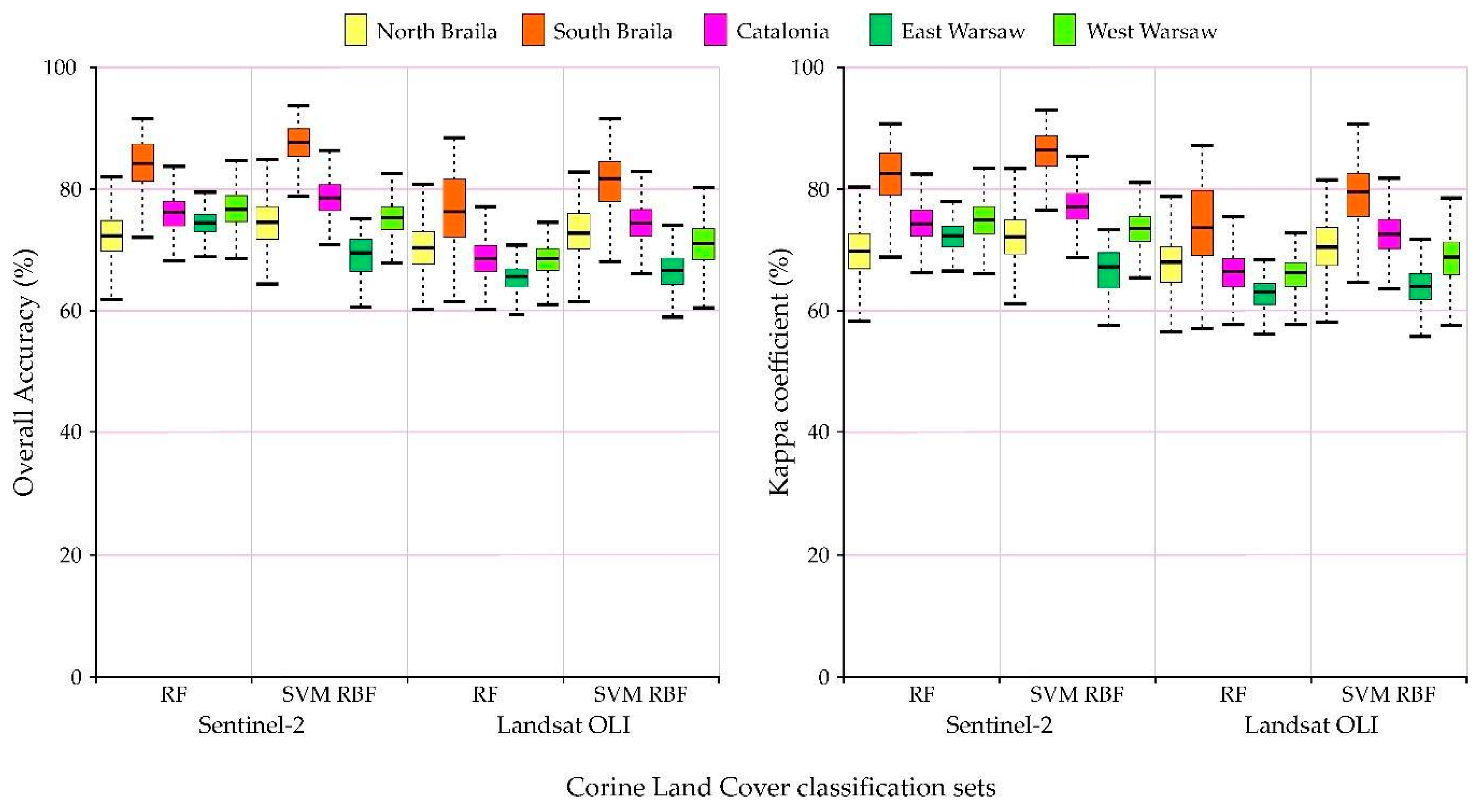
The comparison of accuracy according to the F1-score of individual classes for 100 repetitions of independent classifications is presented in Figure 9, Figure 10, Figure 11 and Figure 12, and the values of the overall accuracy and the Kappa coefficient in Figure 13. The highest values of the median F1-score were obtained for spectrally homogenous classes, e.g., 511 (water courses), 512 (water bodies), and 523 (sea and ocean); coniferous forests (312) and vineyards (221).

Sentinel-2 images could receive higher values of the F1-score median as well as a smaller spread of final results for the categories of anthropogenic land cover than in the case of Landsat 8 images. The OLI scanner’s classification results obtained slightly higher median results for pastures (231) and land principally occupied by agriculture, with significant natural vegetation areas (243).

Individual research areas were characterized by high variability within classes:

• Northern Braila obtained the highest median results for pastures (231), the worst for industrial or commercial units (class 121). It is also worth noting that in the case of classes 511 and 512, Sentinel-2 images classified by Random Forest were characterized by a large range of data distribution, significantly different from other areas.
• Southern Braila area is characterized by large homogeneous areas, which allowed high median scores for: rice fields (213), complex cultivation patterns (242), inland marshes (411); however, scores were poor for the coniferous forest class (312).
• Catalonia obtained the highest median values for continuous urban fabric (111), discontinuous urban fabric (112), as well as for forests (311, 312). In the case of the complex cultivation patterns (242), it obtained low median results in Catalonia.
• Eastern Warsaw areas received high median values for sport and leisure facilities (142), fruit trees, and berry plantations (222), while in the case of transitional woodland-shrub class (324), despite a significant range of data distributions for other areas, the results were the lowest scores obtained.
• Western Warsaw obtained high median results for fruit trees and berry plantations (222) and mixed forests (313). In the case of classification using the Support Vector Machines algorithm in the Landsat 8 imaging, water bodies (512) were characterized by a significant range of data distributions significantly different from the results obtained for other areas.

The lowest median results were obtained for classes such as: olive groves (223), complex cultivation patterns (242), Land principally occupied by agriculture, with significant areas of natural vegetation (243), and transitional woodland-shrubs (324).

All areas obtained satisfactory overall accuracy and Kappa coefficient results (Figure 13). The highest values of the median total accuracy were achieved for the northern area of Braila and the lowest total accuracy was for eastern Warsaw. Regarding the classifiers, the Support Vector Machines with a radial nucleus obtained higher maximum values of the total accuracy and the Kappa coefficient, but they were characterized by a larger spread than the Random Forest. In the case of imaging, higher median values were obtained for the Sentinel-2 satellite data.

In all cases, higher accuracies were obtained using Sentinel-2 images than Landsat 8. In the classifiers for areas in Romania and Catalonia, Support Vector Machines with the RBF turned out to be better. In contrast, for areas located in Poland, higher accuracy was obtained for the Random Forest algorithm.

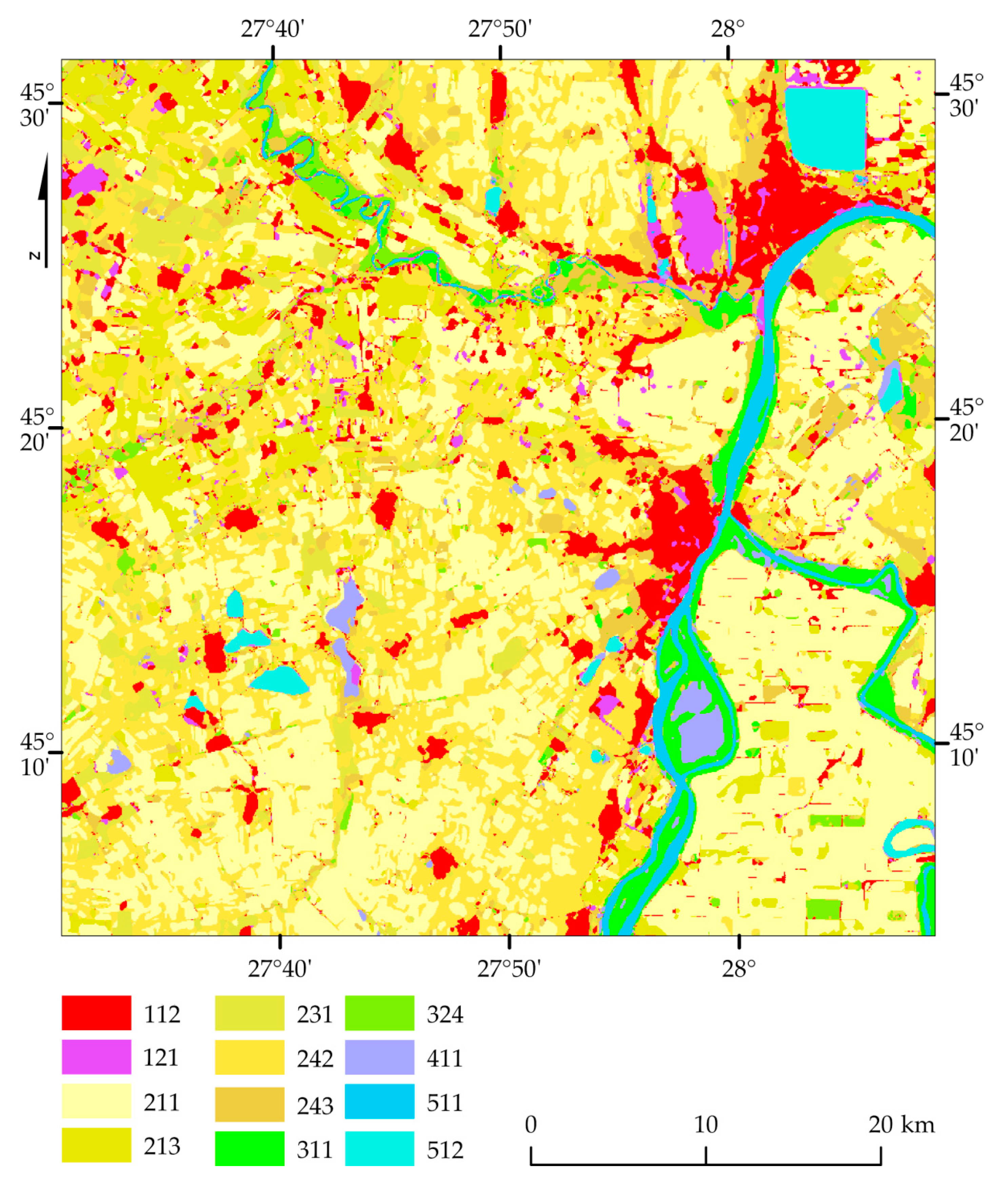
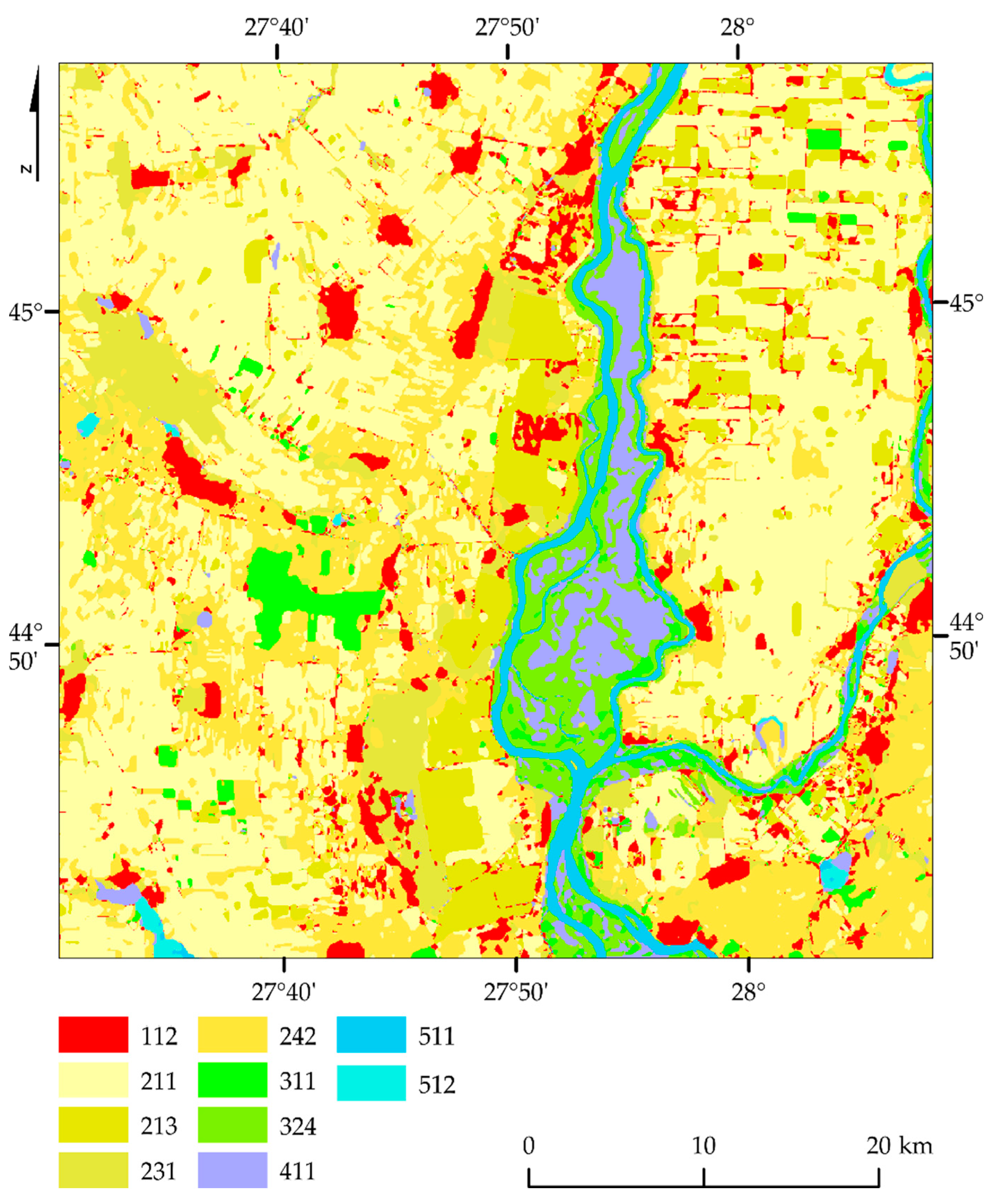
Analyzing the map (Figure 14) and the error matrix (

Table 5. Confusion matrix of the North Braila area (SVM RBF, Sentinel-2 images, overall accuracy (OA): 84%, Kappa coefficient 0.82, UA—User Accuracy, PA—Producer Accuracy, F1-score).

Class	112	121	211	213	231	242	243	311	324	411	511	512	UA	F1
112	421	215	13	0	7	36	13	7	45	51	1	13	51%	64%
121	54	254	15	0	0	16	5	0	41	0	1	0	66%	57%
211	0	5	460	2	0	29	6	1	0	4	0	0	91%	91%
213	0	0	2	491	6	0	0	0	0	0	0	0	98%	98%
231	0	4	0	0	421	3	0	0	0	0	0	0	98%	91%
242	12	17	10	7	22	382	18	1	49	0	0	0	74%	75%
243	9	5	0	0	44	34	453	12	87	3	0	0	70%	79%
311	1	0	0	0	0	0	3	456	0	0	0	0	99%	95%
324	3	0	0	0	0	0	2	21	278	1	0	0	91%	69%
411	0	0	0	0	0	0	0	2	0	441	0	0	100%	94%
511	0	0	0	0	0	0	0	0	0	0	498	0	100%	100%
512	0	0	0	0	0	0	0	0	0	0	0	487	100%	99%
PA	84%	51%	92%	98%	84%	76%	91%	91%	56%	88%	100%	97%

) of the North Braila area, the best results were achieved by water courses (511; F1 100%), water bodies (512; F1 99%), and rice fields (213; F1 98%). The problems were noticed in the case of the transitional woodland-shrub (324; F1 69%), which is often confused with land principally occupied by agriculture, with significant areas of natural vegetation (243) as well as complex cultivation patterns (242). The lowest values were obtained for the building classes: Industrial or commercial units (121; F1 57%) and discontinuous urban fabric (112; F1 64%), often mixing with each other.

Another of the analyzed Romanian areas is Braila district’s southern fragment (granula 35TNK, Figure 15). The area was classified very well due to large and homogenous agriculture areas, e.g., numerous rice fields (213), which were rarely confused with the non-irrigated arable land class (211) in places where there was intensive vegetation and classified very well. Satisfactory results were also obtained for inland marshes (411) and water courses (511). There are similar results as in the case of the northern Braila area (Figure 14); the best results were obtained for the classes of water bodies (512; F1 100%), water courses (511; F1 98%), and inland marshes (411; F1 93%;

Table 6. Confusion matrix of the South Braila area (SVM RBF, Sentinel-2 images, OA: 86%, Kappa coefficient 0.84, UA—User Accuracy, PA—Producer Accuracy, F1-score).

Class	112	211	213	231	242	311	324	411	511	512	UA	F1
112	459	2	0	4	11	101	0	0	0	0	80%	85%
211	9	473	52	9	81	5	0	1	8	0	74%	83%
213	7	12	446	0	0	0	0	0	0	0	96%	92%
231	4	1	0	468	39	0	0	3	3	0	90%	92%
242	20	12	2	1	369	4	0	0	0	0	90%	81%
311	0	0	0	0	0	316	25	25	0	0	86%	73%
324	1	0	0	18	0	71	469	20	5	0	80%	87%
411	0	0	0	0	0	3	6	451	6	0	97%	93%
511	0	0	0	0	0	0	0	0	478	0	100%	98%
512	0	0	0	0	0	0	0	0	0	500	100%	100%
PA	92%	95%	89%	94%	74%	63%	94%	90%	96%	100%

). The complex cultivation patterns class (242) obtained (F1 81%) mixed with the non-irrigated arable land class (211). The lowest results, although relatively high, were achieved by the broad-leaved forest class (311; F1 73%), mixing with discontinuous urban fabric (112) and transitional woodland-shrub (324).

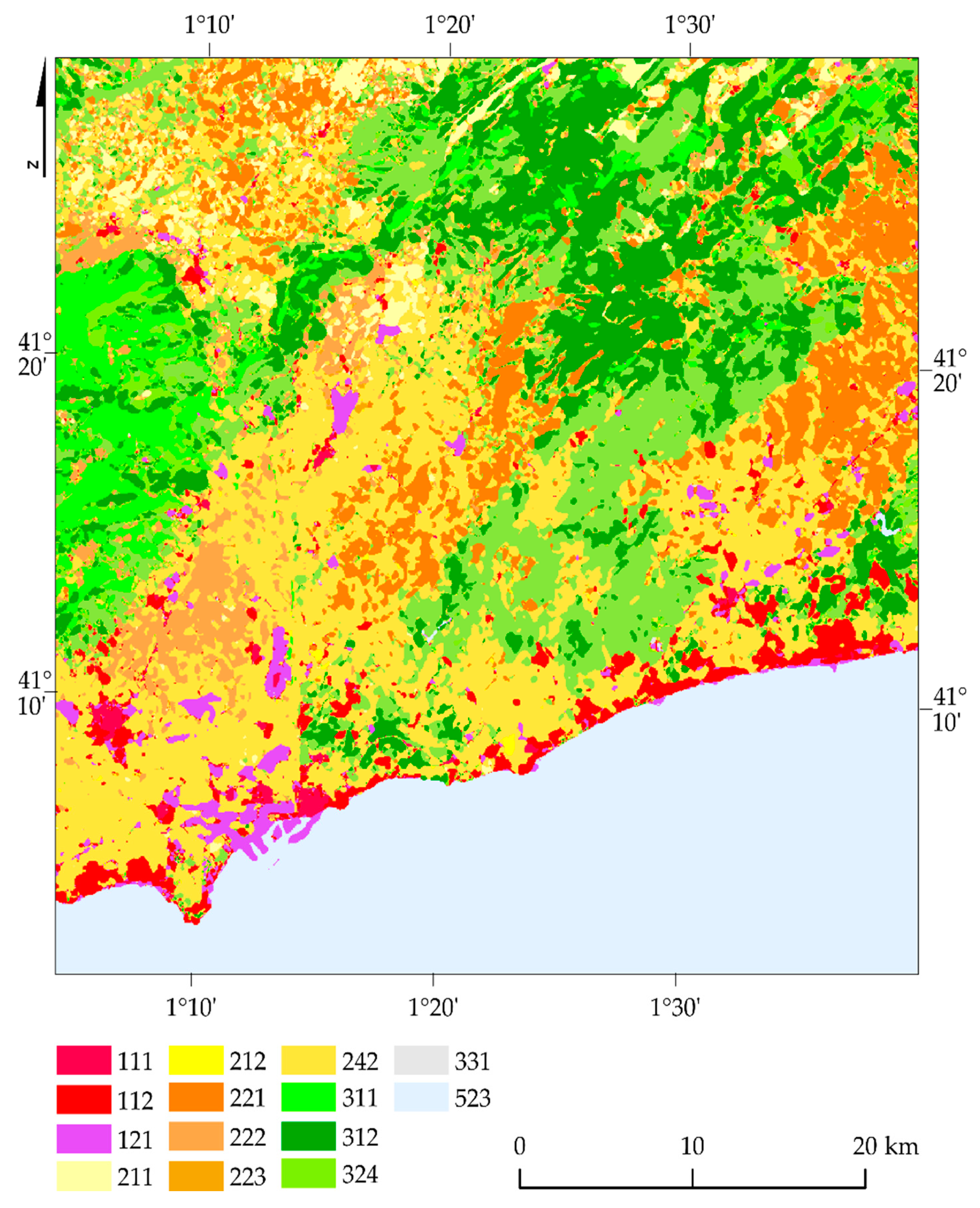
In the case of the Catalonia region (Figure 16), the sea and ocean patterns (523; F1 100%), coniferous forests (312; F1 99%), broad-leaved forest (311; F1 95%), and discontinuous urban fabric (112; F1 95%) were well distinguished (

Table 7. Confusion matrix of the Catalonia area (SVM RBF, Sentinel-2 images, OA: 76%, Kappa coefficient 0.74, UA—User Accuracy, PA—Producer Accuracy, F1-score).

Class	111	112	121	211	212	221	222	223	242	311	312	323	324	331	523	UA	F1
111	428	0	0	0	0	0	0	0	1	0	0	0	0	0	0	100%	92%
112	7	490	0	0	0	0	0	18	16	0	0	0	0	0	0	92%	95%
121	19	0	494	1	7	0	0	0	2	0	0	0	0	387	0	54%	70%
211	0	0	0	458	144	1	0	0	52	0	0	0	0	0	0	70%	79%
212	0	0	0	0	105	0	10	0	12	0	0	0	0	0	0	83%	33%
221	0	0	0	0	15	457	6	0	33	0	0	0	0	0	0	89%	90%
222	0	0	0	2	0	4	426	31	49	0	0	0	0	0	0	83%	84%
223	0	0	0	0	0	2	0	23	10	0	0	0	0	0	0	66%	9%
242	44	9	0	39	226	34	58	397	305	0	0	0	15	0	0	27%	37%
311	0	0	0	0	0	0	0	0	3	492	1	0	43	0	0	91%	95%
312	0	0	0	0	0	0	0	0	0	2	498	0	8	0	0	98%	99%
323	2	1	0	0	3	2	0	25	16	0	1	500	23	0	0	87%	93%
324	0	0	0	0	0	0	0	6	1	6	0	0	411	0	0	97%	89%
331	0	0	6	0	0	0	0	0	0	0	0	0	0	113	0	95%	37%
523	0	0	0	0	0	0	0	0	0	0	0	0	0	0	500	100%	100%
PA	86%	98%	99%	92%	21%	91%	85%	5%	61%	98%	100%	100%	82%	23%	100%

). Vineyards (221), fruit trees, and berry plantations (222) were correctly classified, defining their precise range. Low values were obtained for the class permanently irrigated land (212; F1 33%), often mixing with pixels of non-irrigated arable lands (211) and complex cultivation patterns (242). This happened because there were difficulties identifying it with the olive groves class (223; F1 9%), where the space between individual groves was classified as the class of complex cultivation patterns (242). The beaches, dunes, and sands class (331; F1 37%) also obtained unsatisfactory results, confusing the industrial or commercial units (121).

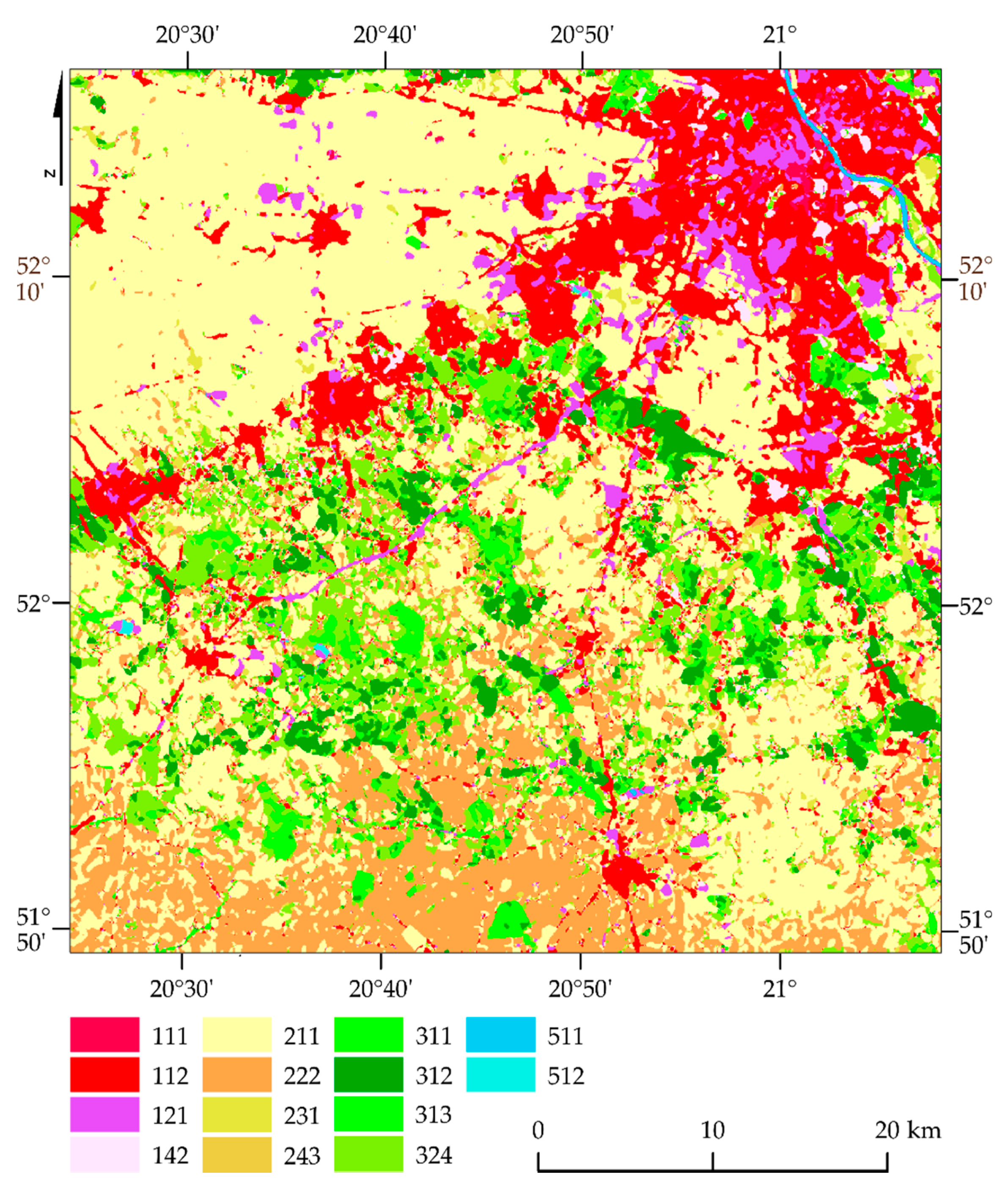
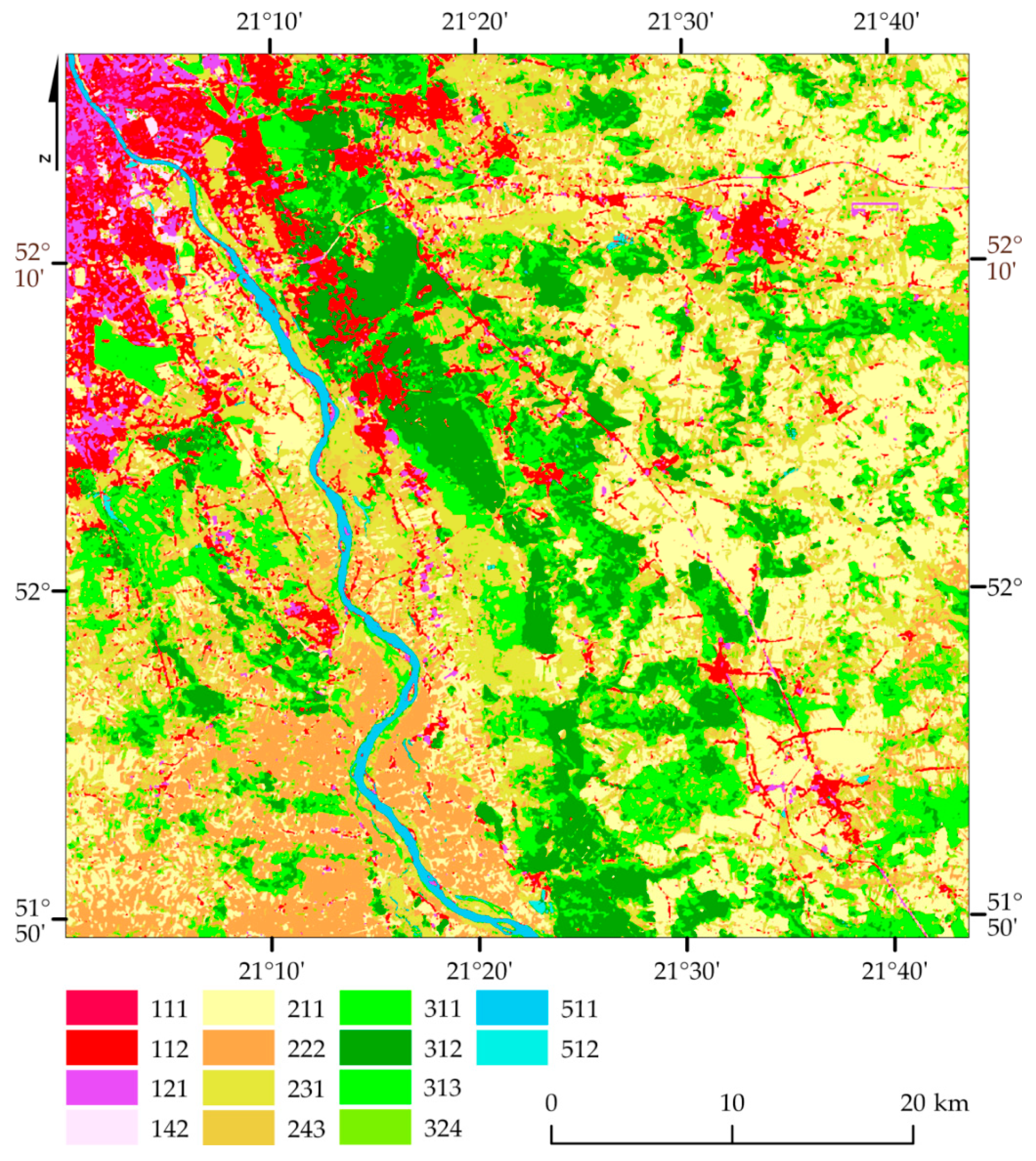
In the case of Polish test areas (western part of Warsaw, granula 35UDC, Figure 17, and eastern Warsaw, granula 35UFC, Figure 18), fruit trees and berry plantations (222), coniferous forest (312), as well as water courses (511) and water bodies (512) are visually the best, creating dense tracts. Sporadically mixed forests (313) were confused with transitional woodland-shrubs (324), with which broad-leaved forest pixels (311) were mixed up often. The pastures (231) and land principally occupied by agriculture, with significant natural vegetation areas (243), were classified in a discontinuous and fragmentary way. Visually, the worst was the class of industrial or commercial units (121), which was often overestimated, and the effect is the strongest in the case of urban fabric (111, 112). The error matrix analysis (

Table 8. Confusion matrix of the West Warsaw area (RF, Sentinel-2 images, OA: 80%, Kappa coefficient 0.78, UA—User Accuracy, PA—Producer Accuracy, F1-score).

Class	111	112	121	142	211	222	231	243	311	312	313	324	511	512	UA	F1
111	469	3	11	0	0	0	0	0	0	0	0	0	0	0	97%	95%
112	31	445	105	35	6	0	0	0	0	0	0	0	0	0	72%	79%
121	0	12	338	0	1	0	0	0	0	0	0	0	0	0	96%	79%
142	0	4	0	257	1	0	0	0	0	0	0	0	0	0	98%	67%
211	0	31	46	9	431	4	61	67	0	0	0	8	0	0	66%	75%
222	0	1	0	108	14	490	0	105	0	0	0	0	0	0	68%	80%
231	0	4	0	50	39	0	397	36	0	0	0	90	0	0	64%	71%
243	0	0	0	7	3	3	0	252	0	0	0	12	0	0	91%	65%
311	0	0	0	0	0	0	0	0	345	0	6	76	0	0	81%	74%
312	0	0	0	0	1	0	0	0	0	481	21	0	0	0	96%	96%
313	0	0	0	0	0	0	0	0	0	9	414	32	0	0	91%	87%
324	0	0	0	34	4	3	42	40	155	10	59	282	0	0	45%	50%
511	0	0	0	0	0	0	0	0	0	0	0	0	500	0	100%	100%
512	0	0	0	0	0	0	0	0	0	0	0	0	0	500	100%	100%
PA	94%	89%	68%	51%	86%	98%	79%	50%	69%	96%	83%	56%	100%	100%

and

Table 9. Confusion matrix of the East Warsaw area (RF, Sentinel-2 images, OA: 80%, Kappa coefficient 0.78, UA—User Accuracy, PA—Producer Accuracy, F1-score).

Class	111	112	121	142	211	222	231	243	311	312	313	324	511	512	UA	F1
111	387	73	110	0	0	0	0	0	0	0	0	0	0	0	68%	72%
112	11	365	29	17	7	0	2	0	0	0	0	0	0	0	85%	78%
121	102	35	360	0	5	0	0	0	0	0	0	0	0	0	72%	72%
142	0	0	0	483	2	0	3	0	0	0	0	0	0	0	99%	98%
211	0	22	1	0	403	8	20	0	0	0	0	10	0	0	87%	84%
222	0	0	0	0	10	468	4	6	0	0	0	43	0	0	88%	91%
231	0	0	0	0	37	3	450	23	0	0	0	2	0	0	87%	89%
243	0	2	0	0	20	4	20	410	12	0	24	325	0	0	50%	62%
311	0	0	0	0	0	0	0	50	434	0	76	34	0	0	73%	79%
312	0	0	0	0	1	15	0	0	0	474	27	0	0	0	92%	93%
313	0	0	0	0	5	0	0	0	43	25	373	80	0	0	71%	73%
324	0	2	0	0	10	2	1	11	11	0	0	6	0	0	14%	2%
511	0	0	0	0	0	0	0	0	0	0	0	0	500	0	100%	100%
512	0	1	0	0	0	0	0	0	0	1	0	0	0	500	100%	100%
PA	77%	73%	72%	97%	81%	94%	90%	82%	87%	95%	75%	1%	100%	100%

) showed the best results were obtained in the classes of water courses (511) and water bodies (512; F1 100%) as well as coniferous forest (312; 96%). Sport and leisure facilities (142) have often been confused with fruit trees and berry plantations (222) and pastures (231). The class land principally occupied by agriculture, with significant areas of natural vegetation (243), was often misassigned to the non-irrigated arable land classes (211) and fruit trees and berry plantations (222). The worst results were transitional woodland-shrubs (324; F1 50%), which were confused with pastures (231) and broad-leaved forest (311).

The applied classification methodology required data acquisition from spring, summer, and autumn, which allowed us to identify most of the classes that occur and automatically be identified, regardless of geographic location (

Table 10. Mean F1-scores of Sentinel-2 image classifications of the best algorithms for each region.

Class Description	Class	Mean F1
Sea and ocean	523	100%
Water courses	511	98%
Water bodies	512	97%
Rice fields	213	96%
Beaches, dunes, sands	331	95%
Vineyards	221	94%
Coniferous forest	312	94%
Permanently irrigated land	212	93%
Sclerophyllous vegetation	323	93%
Inland marshes	411	92%
Broad-leaved forest	311	91%
Pastures	231	90%
Sport and leisure facilities	142	90%
Continuous urban fabric	111	89%
Fruit trees and berry plantations	222	88%
Non-irrigated arable land	211	85%
Discontinuous urban fabric	112	83%
Mixed forest	313	80%
Industrial or commercial units	121	74%
Complex cultivation patterns	242	68%
Land principally occupied by agriculture, with significant areas of natural vegetation	243	67%
Transitional woodland/shrub	324	65%
Olive groves	223	32%

). The problem is the selection of the right number of training and verification pixels (

Table 11. Increases mean OA accuracies under changing the number of pixels.

	Sentinel-2		Landsat 8
Number of Pixels	RF	SVM RBF	RF	SVM RBF
100	73.1%	75.6%	67.1%	68.2%
200	75.4%	76.7%	67.5%	69.0%
300	76.7%	78.0%	69.8%	69.5%
400	77.2%	80.3%	70.3%	71.7%
500	78.3%	81.4%	71.1%	72.4%

), which should be updated regularly, as significant changes were observed between the original Corine map from 2018 and contemporary satellite images, e.g., lack of water in selected water bodies or densely built-up areas instead of green areas.

4. Discussion

In our opinion, there is a lack of comparison of CLC products obtained using different areas, sensors, and classifiers in the literature. We focused on conducting analyzes on individual Sentinel-2 imaging granules, selecting three countries characterized by a different history, which influenced spatial management (starting from large-scale agricultural crops (South Braila), a large urban agglomeration (Warsaw) with direct operating facilities, including the suburban zone, which on the one hand provides protected areas and climatic resorts along Vistula river, as well as typical suburban zones, including small farms providing food for suburban towns), but also coastal and river port areas (Tarragona, North Braila) and well-known tourist areas. The selection of tools was not accidental, because, based on the literature review, we wanted to use machine learning algorithms that are widely available and based on a programming language, which allows us to automate the procedure for classifying subsequent areas. In many cases, the results obtained on the original data (20 m Sentinel-2 and 30 m Landsat 8) were much more accurate than on the generalized data (60 m), and then filtered to a resolution of 480 × 480 m, which is a requirement of Corine Land Cover. In our work, we compared results obtained using four different SVM kernels and the Random Forest classifier. We also included a multi-temporal composition, which gave satisfying results without having to search for additional datasets to make the images more informative (other sensors, radar, lidar, etc.). This is especially important considering adding additional data is time-consuming (especially if the product is developed for the whole of Europe). We investigated the relation between the number of pixels used for training per class and the classifier used. Such works are not rare, but they mostly focus on either problem, not on both as we carry out here. Our results will help inform further CLC+ creators about the required minimum number of pixels per class they need to acquire in order to deliver acceptable results. Our study is particularly relevant now that a new version of CLC+ is being developed, with a heavy focus on creating solutions employing classification approaches that enrich the final product.

Despite the advantages and numerous applications, CLC products and analyses carried out should be treated with caution, and researchers should be aware of the restrictions associated with them [26]. Despite the continuous improvement of definitions, a significant disadvantage is the ambiguity of the class description, as Jansen and Di Gregorio [53] pointed out. Diaz-Pacheco and Gutiérrez [54] highlighted a significant impact of subjective photo interpretation on results, which translates into thematic accuracy, insufficient standardization, and harmonization of data. The difference in thematic accuracy in the scale of regions and countries is also noted by García-Alvarez and Camacho-Olmedo [55]; problems with detailed analyses of land cover were noticed by Di Sabatino et al. [56]. According to the European Environmental Agency [57], the most challenging and subjective classes in photointerpretation are classes: 242, 243, 313, and 324 [57]; in the case of our classifications, it was confirmed only in the case of class 324 (East and West Warsaw) and 242 (Catalonia). The rest of the areas offered an acceptable level of classification accuracies (

Table 12. F1-score indices of heterogeneous classes.

Class	South Braila	North Braila	Catalonia	West Warsaw	East Warsaw
242	81%	75%	37%	-	-
243	-	79%	-	65%	62%
313	-	-	-	87%	73%
324	87%	69%	89%	50%	2%

). It is also worth noting that in 2012 there was a change in the methodology for creating the German CLC [58], which caused a significant decrease in area in classes 242, 243, and an increase in area in class 231. The standard photointerpretation (used in CLC 1990, 2000, and 2006) was replaced by an original methodology based on the use of the existing Digital Land Cover Model for Germany (DLM-DE) national data, which is much more detailed (the size of the minimum mapping unit (MMU) is 1 ha). This makes it impossible to analyze changes between versions with the old and the new methodology. Besides, the CLC technical team verification in many countries has shown that a common mistake in photointerpretation is the overestimation of classes 242 and 243 [59]. The process of creating CLC is time-consuming, expensive, and the final product is published with a significant delay between data collection and publication.

F-score for complex agricultural areas (classes 242 and 243) oscillate around 80% for Brailas (F1: 81%, 75%, 79%), the same accuracies were observed by Denize et al. [60], who used Sentinel-2 data and SVM and RF algorithms for classifying crop residues, bare soil, winter crop, and grassland scoring an overall accuracy of 81%. For the same source of data and Random Forest algorithms for maize, onion, sunflower, and sugar beet, Immitzer et al. [61] achieved 65–76%, which is a similar result to the Warsaw area in our study.

Phiri et al. [62], based on an analysis of 222 papers oriented on land cover mapping, confirmed that SVM and Random Forest algorithms offered the best accuracies in the case of Sentinel-2 images (89–92%) than Landsat-based maps; although the mean classification results of Random Forest and SVM were comparable (~89%), as the maximal, as well (~93–95%) [62]. General observations were confirmed in our case, where we could notice a similar range of the best results, but in our case, SVM RBF obtained results better by two to three percent than RF.

Analyzing the sensor’s effect on classification accuracy, better total accuracy results (7–8%) were obtained for the MSI sensor than OLI regardless of the algorithm used. For the Random Forest a Support Vector Machines algorithm, the differences between the MSI and OLI sensors were 8% and 7% in favor of MSI, respectively. The advantage of the MSI scanner over OLI in overall accuracy (2–8%) was also recognized by Phiri et al. [62], who collated 20 scientific papers on land cover classification. The researchers noted that the MSI scanner was 8% better for the Random Forest algorithm, while for Support Vector Machines the difference was smaller at only 2%. Similar conclusions were also reached by Forkuor et al. [63] by resampling the resolution of Landsat 8 to Sentinel-2 (10 m), obtaining higher overall accuracies (2–4%) for the MSI scanner than OLI. Additionally, when resampling Sentinel-2 to Landsat 8 resolution (30 m), performed by Topaloğlu et al. [64], it led to better total accuracy results (2%) for the MSI scanner than OLI. Despite the longer operational time of the Landsat series of satellites than Sentinel-2, allowing for the development of data processing methods, an important element seems to be the larger number of multispectral bands (Sentinel-2: 13 bands, Landsat 8: 8 bands) of the MSI scanner increasing the classification accuracy (

Table 13. Comparison of the obtained results with the literature.

Author	Number of Classes	Instrument (Spatial Resolution)	Algorithm	Best OA
Demirkan et al. [67]	4	Sentinel-2 MSI (10 m)	RF	85%
			SVM	85%
	6		RF	82%
			SVM	85%
Close et al. [69]	5	Sentinel-2 MSI (10 m)	RF	88%
Thanh Noi, Kappas [70]	6	Sentinel-2 MSI (20 m)	RF	95%
			SVM	95%
Forkuor et al. [63]	7	Landsat 8 OLI (10 m)	RF	90%
			SVM	89%
		Sentinel-2 MSI (10 m)	RF	92%
			SVM	93%
Weinmann, Weidner [68]	7	Sentinel-2 MSI (10 m)	RF	80%
Topaloğlu et al. [64]	8	Landsat 8 OLI (30 m)	SVM	82%
		Sentinel-2 MSI (30 m)	SVM	84%
Our results	14	Landsat 8 OLI (60 m)	RF	72%
	10		SVM	79%
	14	Sentinel-2 MSI (60 m)	RF	80%
	10		SVM	86%

).

An important element affecting land cover classification accuracy is the number of classes identified (Table 13). Increasing the number of land cover classes identified contributes to a decrease and blurring of spectral differences between classes, resulting in decreased classification accuracy [65]. Additionally, an analysis of 64 articles on land cover classification by the team of Thinh [66] highlights a significant decrease in the total accuracy when increasing the number of classes. In the present study, the highest accuracies were obtained for areas where 10 and 14 classes were present, which significantly affected the classification accuracy and contributed to the differences in the results obtained from other authors who usually designated fewer classes; however, it is not only the number of classes determined that matters, but also the choice of methods for processing the data and making them more informative. Demirkan et al. [67], although identifying only four first-level Corine classes, achieved weaker results than the vast majority of other researchers identifying more classes. The reason for the more inferior result could be the use of only a single satellite image. An acceptable way to increase the data’s informativeness is to create a multi-temporal composition from satellite images acquired at different times. This allows us to not only reduce the influence of a single image and errors that may occur in it, but especially helps to distinguish vegetation types that change their spectral reflectance depending on the analyzed period. In this paper, a multi-temporal composition was used from satellite images acquired in spring, summer, and autumn; however, there are “denser” time series in the literature, as in the case of the team of Forkuor et al. [63], who used Sentinel-2 and Landsat 8 imagery from five dates, obtaining high total accuracy results (89–93%). Increasing the time series does not always produce higher classification accuracy results as shown by the study of Weinmann and Weidner [68] who, using imagery acquired by the MSI scanner for four dates with a small area (16 × 16 km²) and the same number of classes, obtained total accuracy results of up to 80%. It is worth noting that it is impossible for many areas to acquire satellite imagery due to the cloud cover present, which makes analysis impossible.

Another important aspect of differences in classification accuracy is the spatial resolution of satellite data used. On the one hand, the high spatial resolution allows the classification of land cover forms with high precision; on the other hand, land cover requires generalization. That is why many classification systems such as Corine Land Cover allow for the presence of another class in a given class of elements, e.g., farm buildings in agricultural areas, technical paths in forests, and small water bodies in forests. Such generalization is often possible by resampling satellite data to a lower resolution, allowing mixed upland cover classes to occur sporadically within large homogeneous classes. Researchers obtain similar results for several classes regardless of whether they use a higher [69] or lower resolution [64]; however, for the classification of the third level Corine Land Cover data, it was necessary to lower the resolution in order to generalize the land cover classes, allowing a dozen classes to obtain results comparable to other authors. Similar methods are used to identify dozens of Corine classes, as exemplified by the study carried out by Novillo et al. [20], who used 275 m resolution MISR scanner imagery for this purpose, but this was at the cost of reduced precision in class boundary delineation.

Comparing the classifiers used in this study, higher results were obtained for Support Vector Machines than Random Forest for both MSI and OLI scanners (6% and 7% higher, respectively). For the results obtained by Demirkan et al. [67] for four classes, the accuracy differences do not appear in the comparison made by Thanh Noi and Kappas [66]. Only at six classes, a slight advantage in classification accuracy (by 3%) of Support Vector Machines over Random Forest is seen. Slight differences are also found by Forkuor et al. [63], where for the OLI scanner Random Forest is 1% better, and for MSI, there is an inverse relationship where the Support Vector Machines algorithm is 1% better. Phiri et al. [62] found a 4% advantage of Support Vector Machines for the OLI scanner. The MSI scanner Random Forest was found to be 5% better than SVM. The process of selecting hyperparameters for the classifiers, as well as the nature of the data and the number of classes, may have influenced the discrepancies.

Analyzing the results obtained for each Corine level 3 class (

Table 14. Comparison of the obtained results by CLC classes with the literature.

	Baltzer et al. [14]		Gudmann et al. [71]		Our Results
Class	PA	UA	PA	UA	Min. PA	Min. UA	Max. PA	Max. UA
111	75%	39%	-	-	72%	72%	94%	97%
112	77%	77%	84%	73%	77%	68%	98%	92%
121	-	-	46%	68%	51%	66%	99%	54%
142	-	-	15%	95%	51%	98%	97%	99%
211	76%	85%	97%	70%	81%	87%	95%	74%
221	-	-	31%	100%	91%	89%	91%	89%
222	-	-	24%	92%	85%	83%	98%	68%
231	-	-	41%	62%	79%	64%	90%	87%
242	-	-	34%	49%	61%	27%	76%	74%
243	-	-	26%	46%	50%	91%	82%	50%
311	67%	71%	92%	64%	63%	86%	98%	91%
312	70%	79%	58%	81%	95%	92%	100%	98%
313	56%	42%	45%	59%	75%	71%	83%	91%
324	50%	11%	42%	55%	56%	91%	82%	97%
411	-	-	16%	96%	88%	100%	90%	93%
512	-	-	44%	95%	97%	100%	100%	100%

) and comparing them with other authors should be considered satisfactory. Since the classification was carried out in three different study areas, where geographical variability could have significantly influenced the obtained values, we decided to give the minimum and maximum value obtained for a given class from these areas. In the case of anthropogenic sites for classes 111 and 112, a minimum producer accuracy (72% and 77%, respectively) was obtained, comparable to the results of 75% and 77% from Balzter et al. [14]. Despite the use of different methods by the team of Balzter [14], who used Sentinel 1A radar imagery combined with SRTM data, this shows the possibility of successfully classifying development areas for Corine Land Cover. In the case of class 211 agricultural land, the obtained producer accuracies by Gudmann et al. [71] are remarkably high (97%), being slightly higher than the obtained maximum accuracies (95%) for this class. This may have been influenced by the small study area (500 km²) being five times smaller than each study area in this paper, and also the geographical nature of the area may have influenced the result. In the case of classes 242 and 243, where difficulties in classification were encountered, resulting in 61% and 50% of the producer’s minimum accuracy, respectively. Problems in their classification were also found by the team of Gudmann et al. [71], who obtained 34% and 26% of the producer’s accuracy, respectively. This may indicate the inability to identify these classes, and the need to find other methods to classify them effectively is urgent. Additionally, for class 324, the weakest result was obtained (min. PA 56%), which is comparable to other researchers (50% [14]; 42% [71]). For deciduous forests (311), a comparable result (min. PA 63%) was obtained with Balzter et al. [14] (PA 67%). Noticeable differences were found for the coniferous forest class (312), for which the minimum value of the producer’s accuracy (95%) differs significantly from the results obtained by the researchers (70% [14], 58% [71]). The difference of the result in the case of Baltzer et al. [14] can be understood by different characteristics of the radar data, but in the case of the team of Gudmann et al. [71], it differs significantly despite the use of a multi-temporal composition from images acquired by the Sentinel-2 satellite and the Random Forest algorithm. Significant differences are also found for the producer accuracy score (44%) for water bodies (512) obtained by Gudmann et al. [71]. Surprisingly, the low accuracy in particular of the characteristic spectral reflectance curve for water, the rarely occurring problems in identifying this class [72], and the lack of occurrence of other classes related to water areas. The differences obtained may have been influenced by the nature of the study area and its size.

Regarding a usage of more sophisticated classifiers such as those based on deep learning methods, there is a multitude of approaches one can select; simple implementations such as a deep multilayered perceptron offers comparable results as obtained by SVM or RF, but optimizing procedure requires more time and better servers [72]. In order to compare shallow and deep learning methods, it is necessary to prepare the data in an appropriate way to compare them objectively (Liu, 2017) [73], also bias can be introduced without following uniform rules, where often one method is favored and its parameters optimized, while other algorithms are not optimized and are assigned default parameter values [74]. Additionally, it should be emphasized that for deep learning methods a very large number of samples were needed for training which requires more computing resources and longer time for optimizing the parameters [73]. In our case, the challenge for the classifiers was to determine patterns of the same classes, but biogeographically different areas, where different spatial management principles apply. For example, research carried out by Ulmas and Liiv (2020) [72] where a convolutional machine learning model with a modified U-Net structure was used to classify land cover according to Corine Land Cover nomenclature did not yield better results, e.g., lowest results were obtained for the classes: discontinuous urban fabric (class 112; F1-score: 1%, and in our case the lowest 42% for Landsat 8, in case of Sentinel-2 results were better; Figure 9, Figure 10, Figure 11 and Figure 12), industrial or commercial units (class 121; F1-score: 36%, and in our case 4%), sport and leisure facilities (class: 142; F1 0%, and in our case 42%), rice fields (class 213; F1 12%, and in our case 42%), fruit trees and berry plantations (class 222; F1 27%, and in our case 28%). Additionally, for water area classes where there are usually no problems with their classification low accuracies were obtained (F1 38-83%, and we observed the lowest accuracy in Warsaw’s 8%, but its median achieved 84% (class 512), excluding this one case, the lowest accuracy scored 48%, but the lowest median 84%). Additionally, the superiority of deep learning methods over Random Forest and Support Vector Machines was not observed in other land cover classification studies [74,75]. Naturally, this is a subject of discussion since much depends on the subject of classification (number of classes, data, how distinct classes are, etc.). Most works focus on using artificial neural networks and their variations to classify datasets structured in the same way as for SVM or RF [76,77,78,79]. That is, to classify images using pixel-based approaches. This approach disregards the natural advantages of more advanced deep learning techniques such as convolutional or deconvolutional neural networks, which can exploit relations between pixels and objects on the image [73]. Proper use of those advantages allows for more accurate results that are also easier to analyze (such as providing class labels to image parts instead of individual pixels) [80]. Moreover, when deciding to investigate deep learning, one must be ready to invest a significant amount of time into processing and training steps. The use of deep learning enormously increases processing times compared to classical machine learning algorithms [81], especially when large areas are involved. This, combined with the expertise required by deep learning, leads to interesting but challenging problems that are yet to be thoroughly investigated.

5. Conclusions

The result of the work is the verification of the potential of both the Landsat 8 images that formed the basis of the Corine program and the Sentinel-2 data. The conducted analyzes showed a several percent advantage of the Sentinel-2 data, despite the fact that the classification was carried out on the basis of resampled data to a resolution of 60 m. Another key result is the analysis of the usefulness of algorithms. The Support Vector Machine algorithm with the radial kernel function (SVM RBF) achieved significant results for all research areas. The following part focused on this classifier and Random Forest, making the prediction of the result images on both Sentinel-2 and Landsat 8 imagery. SVM results are characterized by a smaller range of data distributions such as deciduous forests (311), water courses (511), and water bodies (512) than in the case of the results obtained for Random Forest, which, however, obtained a smaller range of data distribution for permanently irrigated land (211). Comparing the classification images with the original Corine Land Cover study shows that more detail is included, which makes the class areas less homogeneous than in the original study. There is also a difference in the degree of generalization between results acquired from the Landsat 8 and Sentinel-2 imagery. The performed analyzes confirmed that the presented results are not the best that can be obtained based on the RF and SVM algorithms and the used data, higher results were obtained for the original resolutions (20 m Sentinel-2 and 30 m Landsat 8), but the Corine program guidelines required generalization to a resolution of 500 × 500 m (in our case we used 480 × 480 m), which lowered the presented results by several percent. Sentinel-2 shows the land cover in more detail, offering 8–11% higher results, e.g., a particularly big difference can be observed for the areas of South and North Braila. Random Forest classifier better generalized agricultural areas than Support Vector Machines, which classified technical objects and some roads as class 112 (industrial or commercial units). For research areas in Romania, there are significant differences in the share of class 242 (complex cultivation patterns, which in the original study was strongly underestimated) at the expense of class 211 (non-irrigated arable land). As for the area of northern Braila, there is a discrepancy in the identification of water reservoirs (class 512), which remained without water during the satellite imaging.

Concerning the area of Catalonia, the original study by Corine Land Cover, there was a significant change in the share of classes 221 (vineyards) and 222 (fruit trees and berry plantations) in favor of class 242 (complex cultivation patterns), indicating their distribution in more detail. Considerable differences in the classification of the above-mentioned classes can be seen between the Sentinel-2 and Landsat 8 images. The changes can also be seen in the forest type area where the coniferous forest area (312) has decreased in favor of deciduous forests (311). In the Catalonia area, the building classes were very well distinguished: 111 (continuous urban fabric), 112 (discontinuous urban fabric), and 121 (industrial or commercial units). In the case of Warsaw areas, orchard areas (222) represented the very well-classified class. As in Catalonia, the different forest classes (311, 312, and 313) were mapped in more detail than in the original CLC study. The Sentinel-2 images show the orchard class (222) in more detail than the Landsat images. Difficulties were noticed in distinguishing classes 111 (continuous urban fabric) and 121 (industrial or commercial units), because it is a class with small areas with very closed pixels values so that the thresholding process of pixels representing is very confused and given classes mixed with each other, characterized by large granularity, discontinuity, and mosaic character. The survey carried out although three test areas in different parts of Europe is still a small area in comparison to the whole European area, so it is necessary to investigate further areas and check individual combinations of classes. In this study, a total of 23 out of 44 Corine coverage classes were checked. Due to the nature of the area, given classes may obtain lower or higher accuracy depending on the co-occurrence of classes with similar terrain characteristics. Results from this research could help Corine Land Cover+ producers with decisions related to selecting algorithms, satellite data, and the possibilities and difficulties of classifying individual Corine Land Cover classes. This study indicates that Corine Land Cover classes could be classified with high accuracy.

The most important conclusions from the study are:

• Sentinel-2 satellite images allowed to classify land cover with better overall accuracy (8–10%) than the Landsat 8 data,
• Support Vector Machines algorithm with an RBF kernel function achieved the best results and obtained higher overall accuracy results (6–7%) than Random Forest,
• the best classification results were achieved for classes: Sea and ocean (523, F1: 100%), water courses (511, F1: 98%), water bodies (512, F1: 97%), rice fields (213, F1: 96%), beaches, dunes, sands (331, F1: 95%), vineyards (221, F1: 94%), coniferous forests (312; F1: 94%), permanently irrigated lands (212, F1: 93%), sclerophyllous vegetation (323, F1: 93%), inland marshes (411, F1: 92%), broad-leaved forest (311, F1: 91%), pastures (231, F1: 90%), and sport and leisure facilities (142, F1: 90%),
• classes characterized by discontinuity and fragmentation obtained lower accuracy results than compact homogeneous large-area classes,
• the difficulties in classification were found in heterogeneous classes, containing many elements of coverage simultaneously, e.g., industrial or commercial units (121, F1: 74%), complex cultivation patterns (242, F1: 68%), land principally occupied by agriculture, with significant areas of natural vegetation (243, F1: 67%), transitional woodland/shrubs (324, F1: 65%), and olive groves (223, F1: 32%).

References

1. Congalton, R.; Gu, J.; Yadav, K.; Thenkabail, P.; Ozdogan, M. Global Land Cover Mapping: A Review and Uncertainty Analysis. Remote Sens. 2014, 6, 12070–12093. [Google Scholar] [CrossRef] [Green Version]
2. Karpatne, A.; Jiang, Z.; Vatsavai, R.R.; Shekhar, S.; Kumar, V. Monitoring Land-Cover Changes: A Machine-Learning Perspective. IEEE Geosci. Remote Sens. Mag. 2016, 4, 8–21. [Google Scholar] [CrossRef]
3. Olofsson, P.; Foody, G.M.; Herold, M.; Stehman, S.V.; Woodcock, C.E.; Wulder, M.A. Good practices for estimating area and assessing accuracy of land change. Remote Sens. Environ. 2014, 148, 42–57. [Google Scholar] [CrossRef]
4. Büttner, G.; Kosztra, B. CLC2018 Technical Guidelines; Service Contract No 3436/R0-Copernicus/EEA.56665; European Environment Agency: Wien, Austria, 2017; p. 61. [Google Scholar]
5. Fernández-Nogueira, D.; Corbelle-Rico, E. Determinants of Land Use/Cover Change in the Iberian Peninsula (1990–2012) at Municipal Level. Land 2019, 9, 5. [Google Scholar] [CrossRef] [Green Version]
6. Pekkarinen, A.; Reithmaier, L.; Strobl, P. Pan-European forest/non-forest mapping with Landsat ETM+ and CORINE Land Cover 2000 data. ISPRS J. Photogramm. Remote Sens. 2009, 64, 171–183. [Google Scholar] [CrossRef]
7. Janssen, S.; Dumont, G.; Fierens, F.; Mensink, C. Spatial interpolation of air pollution measurements using CORINE land cover data. Atmos. Environ. 2008, 42, 4884–4903. [Google Scholar] [CrossRef]
8. Gallego, F.J.; Batista, F.; Rocha, C.; Mubareka, S. Disaggregating population density of the European Union with CORINE land cover. Int. J. Geogr. Inf. Sci. 2011, 25, 2051–2069. [Google Scholar] [CrossRef]
9. Stathopoulou, M.; Cartalis, C.; Keramitsoglou, I. Mapping micro-urban heat islands using NOAA/AVHRR images and CORINE Land Cover: An application to coastal cities of Greece. Int. J. Remote Sens. 2004, 25, 2301–2316. [Google Scholar] [CrossRef]
10. Heinl, M.; Walde, J.; Tappeiner, G.; Tappeiner, U. Classifiers vs. input variables—The drivers in image classification for land cover mapping. Int. J. Appl. Earth Obs. Geoinf. 2009, 11, 423–430. [Google Scholar] [CrossRef]
11. Leinenkugel, P.; Deck, R.; Huth, J.; Ottinger, M.; Mack, B. The Potential of Open Geodata for Automated Large-Scale Land Use and Land Cover Classification. Remote Sens. 2019, 11, 2249. [Google Scholar] [CrossRef] [Green Version]
12. Mellor, A.; Boukir, S. Exploring diversity in ensemble classification: Applications in large area land cover mapping. ISPRS J. Photogramm. Remote Sens. 2017, 129, 151–161. [Google Scholar] [CrossRef]
13. Hansen, M.C.; Loveland, T.R. A review of large area monitoring of land cover change using Landsat data. Remote Sens. Environ. 2012, 122, 66–74. [Google Scholar] [CrossRef]
14. Balzter, H.; Cole, B.; Thiel, C.; Schmullius, C. Mapping CORINE Land Cover from Sentinel-1A SAR and SRTM Digital Elevation Model Data using Random Forests. Remote Sens. 2015, 7, 14876–14898. [Google Scholar] [CrossRef] [Green Version]
15. Griffiths, P.; Nendel, C.; Hostert, P. Intra-annual reflectance composites from Sentinel-2 and Landsat for national-scale crop and land cover mapping. Remote Sens. Environ. 2019, 220, 135–151. [Google Scholar] [CrossRef]
16. Jensen, J.R. Introductory Digital Image Processing: A Remote Sensing Perspective, 4th ed.; Pearson: London, UK, 2015; p. 656. ISBN 978-0-13-405816-0. [Google Scholar]
17. Zoungrana, B.J.-B.; Conrad, C.; Amekudzi, L.K.; Thiel, M.; Da, E.D.; Forkuor, G.; Löw, F. Multi-Temporal Landsat Images and Ancillary Data for Land Use/Cover Change (LULCC) Detection in the Southwest of Burkina Faso, West Africa. Remote Sens. 2015, 7, 12076–12102. [Google Scholar] [CrossRef] [Green Version]
18. Gounaridis, D.; Apostolou, A.; Koukoulas, S. Land cover of Greece, 2010: A semi-automated classification using random forests. J. Maps 2016, 12, 1055–1062. [Google Scholar] [CrossRef]
19. Ghamisi, P.; Gloaguen, R.; Atkinson, P.M.; Benediktsson, J.A.; Rasti, B.; Yokoya, N.; Wang, Q.; Hofle, B.; Bruzzone, L.; Bovolo, F.; et al. Multisource and Multitemporal Data Fusion in Remote Sensing: A Comprehensive Review of the State of the Art. IEEE Geosci. Remote Sens. Mag. 2019, 7, 6–39. [Google Scholar] [CrossRef] [Green Version]
20. Novillo, C.; Arrogante-Funes, P.; Romero-Calcerrada, R. Improving Land Cover Classifications with Multiangular Data: MISR Data in Mainland Spain. Remote Sens. 2018, 10, 1717. [Google Scholar] [CrossRef] [Green Version]
21. Sheykhmousa, M.; Mahdianpari, M.; Ghanbari, H.; Mohammadimanesh, F.; Ghamisi, P.; Homayouni, S. Support Vector Machine Versus Random Forest for Remote Sensing Image Classification: A Meta-Analysis and Systematic Review. IEEE J. Sel. Top. Appl. Earth Obs. Remote Sens. 2020, 13, 6308–6325. [Google Scholar] [CrossRef]
22. Rodriguez-Galiano, V.F.; Ghimire, B.; Rogan, J.; Chica-Olmo, M.; Rigol-Sanchez, J.P. An assessment of the effectiveness of a random forest classifier for land-cover classification. ISPRS J. Photogramm. Remote Sens. 2012, 67, 93–104. [Google Scholar] [CrossRef]
23. Janitza, S.; Hornung, R. On the overestimation of random forest’s out-of-bag error. PLoS ONE 2018, 13, e0201904. [Google Scholar] [CrossRef] [PubMed]
24. Gómez, C.; White, J.C.; Wulder, M.C. Optical remotely sensed time series data for land cover classification: A review. ISPRS J. Photogramm. Remote Sens. 2016, 116, 55–72. [Google Scholar] [CrossRef] [Green Version]
25. Golenia, M.; Zagajewski, B.; Ochtyra, A.; Hościło, A. Semiautomatic land cover mapping according to the 2nd level of the Corine Land Cover legend. Polish Cartogr. Rev. 2015, 47, 203–212. [Google Scholar] [CrossRef] [Green Version]
26. Bielecka, E.; Jenerowicz, A. Intellectual Structure of CORINE Land Cover Research Applications in Web of Science: A Europe-Wide Review. Remote Sens. 2019, 11, 2017. [Google Scholar] [CrossRef] [Green Version]
27. Vorovencii, I. Assessing and monitoring the risk of land degradation in Baragan Plain, Romania, using spectral mixture analysis and Landsat imagery. Environ. Monit. Assess. 2016, 188, 439. [Google Scholar] [CrossRef] [PubMed]
28. Bandoc, G.; Prăvălie, R. Climatic water balance dynamics over the last five decades in Romania’s most arid region, Dobrogea. J. Geogr. Sci. 2015, 25, 1307–1327. [Google Scholar] [CrossRef]
29. Boccacci, P.; Botta, R. Microsatellite variability and genetic structure in hazelnut (Corylus avellana L.) cultivars from different growing regions. Sci. Hortic. 2010, 124, 128–133. [Google Scholar] [CrossRef]
30. Rovira, J.; Schuhmacher, M.; Nadal, M.; Domingo, J.L. Contamination by Coal Dust in the Neighborhood of the Tarragona Harbor (Catalonia, Spain): A Preliminary Study. Open Atmos. Sci. J. 2018, 12, 14–20. [Google Scholar] [CrossRef]
31. Traczyk, A. Gospodarstwa sadownicze jako zasób lokalny rozwoju ws iw powiecie grójeckim = Orchard holdings as a local potential for rural development in Grójec county. Stud. Obsz. Wiej. 2017, 47, 99–111. [Google Scholar] [CrossRef]
32. Holnicki, P.; Kałuszko, A.; Nahorski, Z.; Stankiewicz, K.; Trapp, W. Air quality modeling for Warsaw agglomeration. Arch. Environ. Prot. 2017, 43, 48–64. [Google Scholar] [CrossRef] [Green Version]
33. Podawca, K.; Karsznia, K.; Zawrzykraj, A.P. The assessment of the suburbanisation degree of Warsaw Functional Area using changes of the land development structure. Misc. Geogr. 2019, 23, 215–224. [Google Scholar] [CrossRef] [Green Version]
34. Richter, R.; Schläpfer, D. Atmospheric/Topographic Correction for Satellite Imagery; ATCOR-2/3 User Guide, Version 9.0.2 (DLR-IB 565-01/15); DLR—German Aerospace Center: Wessling, Germany; ReSe Applications: Wil SG, Switzerland, 2016; p. 263. [Google Scholar]
35. Mayer, B.; Kylling, A. Technical note: The libRadtran software package for radiative transfer calculations—Description and examples of use. Atmos. Chem. Phys. 2005, 5, 1855–1877. [Google Scholar] [CrossRef] [Green Version]
36. Vermote, E.; Justice, C.; Claverie, M.; Franch, B. Preliminary analysis of the performance of the Landsat 8/OLI land surface reflectance product. Remote Sens. Environ. 2016, 185, 46–56. [Google Scholar] [CrossRef]
37. Stehman, S.V.; Foody, G.M. Key issues in rigorous accuracy assessment of land cover products. Remote Sens. Environ. 2019, 231, 111199. [Google Scholar] [CrossRef]
38. Caret: Classification and Regression Training. R package version 6.0-86. Available online: https://rdrr.io/cran/caret/ (accessed on 25 April 2020).
39. Gaujoux, R. Rngtools: Utility Functions for Working with Random Number Generators. R Package Version 1.5. 2020. Available online: https://rdrr.io/rforge/rngtools/ (accessed on 25 April 2020).
40. Wickham, H.; François, R.; Henry, L.; Müller, K. Dplyr: A Grammar of Data Manipulation. R Package Version 1.0.0. 2020. Available online: https://rdrr.io/cran/dplyr/ (accessed on 25 April 2020).
41. Hijmans, R.J. Raster: Geographic Data Analysis and Modeling. R Package Version 3.3-13. 2020. Available online: https://rdrr.io/cran/raster/ (accessed on 25 April 2020).
42. Bivand, R.; Keitt, T.; Rowlingson, B. Rgdal: Bindings for the ‘Geospatial’ Data Abstraction Library. R Package Version 1.5-12. 2020. Available online: https://rdrr.io/cran/rgdal/ (accessed on 25 April 2020).
43. Liaw, A.; Wiener, M. RandomForest: Classification and Regression by randomForest. R News 2002, 2, 18–22. Available online: https://rdrr.io/cran/randomForest/ (accessed on 25 April 2020).
44. Belgiu, M.; Drăguţ, L. Random forest in remote sensing: A review of applications and future directions. ISPRS J. Photogramm. Remote Sens. 2016, 114, 24–31. [Google Scholar] [CrossRef]
45. Meyer, D.; Dimitriadou, E.; Hornik, K.; Weingessel, A.; Leisch, F. e1071: Misc Functions of the Department of Statistics, Probability Theory Group; (Formerly: E1071); R Package Version 1.7-3; TU: Wien, Austria, 2019; Available online: https://rdrr.io/rforge/e1071/ (accessed on 25 April 2020).
46. Microsoft; Weston, S. doParallel: Foreach Parallel Adaptor for the ‘parallel’ Package. R Package Version 1.0.15. 2019. Available online: https://rdrr.io/rforge/doParallel/ (accessed on 25 April 2020).
47. Microsoft; Weston, S. Foreach: Provides Foreach Looping Construct. R Package Version 1.5.0. 2020. Available online: https://rdrr.io/github/lepennec/foreach/ (accessed on 25 April 2020).
48. Congalton, R.G. A review of assessing the accuracy of classifications of remotely sensed data. Remote Sens. Environ. 1991, 37, 35–46. [Google Scholar] [CrossRef]
49. Pontius, R.G.; Millones, M. Death to Kappa: Birth of quantity disagreement and allocation disagreement for accuracy assessment. Int. J. Remote Sens. 2011, 32, 4407–4429. [Google Scholar] [CrossRef]
50. Foody, G.M. Explaining the unsuitability of the kappa coefficient in the assessment and comparison of the accuracy of thematic maps obtained by image classification. Remote Sens. Environ. 2020, 239, 111630. [Google Scholar] [CrossRef]
51. Hand, D.; Christen, P. A note on using the F-measure for evaluating record linkage algorithms. Stat. Comput. 2018, 28, 539–547. [Google Scholar] [CrossRef] [Green Version]
52. Sabat-Tomala, A.; Raczko, E.; Zagajewski, B. Comparison of Support Vector Machine and Random Forest Algorithms for Invasive and Expansive Species Classification Using Airborne Hyperspectral Data. Remote Sens. 2020, 12, 516. [Google Scholar] [CrossRef] [Green Version]
53. Jansen, L.J.M.; Di Gregorio, A. Parametric land cover and land-use classifications as tools for environmental change detection. Agric. Ecosyst. Environ. 2002, 91, 89–100. [Google Scholar] [CrossRef]
54. Diaz-Pacheco, J.; Gutiérrez, J. Exploring the limitations of CORINE Land Cover for monitoring urban land-use dynamics in metropolitan areas. J. Land Use Sci. 2014, 9, 243–259. [Google Scholar] [CrossRef]
55. García-Álvarez, D.; Camacho Olmedo, M.T. Changes in the methodology used in the production of the Spanish CORINE: Uncertainty analysis of the new maps. Int. J. Appl. Earth Obs. Geoinf. 2017, 63, 55–67. [Google Scholar] [CrossRef]
56. Di Sabatino, A.; Coscieme, L.; Vignini, P.; Cicolani, B. Scale and ecological dependence of ecosystem services evaluation: Spatial extension and economic value of freshwater ecosystems in Italy. Ecol. Indic. 2013, 32, 259–263. [Google Scholar] [CrossRef]
57. Büttner, G.; Maucha, G. The Thematic Accuracy of Corine Land Cover 2000, Assessment using LUCAS (Land Use/Cover Area Frame Statistical Survey); EEA Technical report No 7/2006; European Environmental Agency: Copenhagen, Denmark, 2006; p. 90. ISBN 92-9167-844-9. [Google Scholar]
58. Keil, M.; Esch, T.; Feigenspan, S.; Marconcini, M.; Metz, A.; Ottinger, M.; Zeidler, J. Creation of a high-resolution product CLC2006_backdating by a backward look from the digital land cover model DLM-DE2009 to 2006—A contribution to the German Corine Land Cover 2012 project within a bottom-up approach. ISPRS Int. Arch. Photogramm. Remote Sens. Spat. Inf. Sci. 2015, 1093–1100. [Google Scholar] [CrossRef] [Green Version]
59. Jaffrain, G.; Sannier, C.h.; Pennec, A.; Dufourmont, H.; Bossard, M.; Feranec, J.; Di Federico, A. GMES Initial Operations/Copernicus Land Monitoring Services—Validation of Products (Second Specific Contract) Validation Services for the Geospatial Products of the Copernicus land Continental and Local Components including In-Situ Data (lot 1). Corine Land Cover 2012 Final Validation Report; Prime Contractor: Villeneuve-d’Ascq, France, 2017; p. 214. [Google Scholar]
60. Denize, J.; Hubert-Moy, L.; Corgne, S.; Betbeder, J.; Pottier, E. Identification of winter land use in temperate agricultural landscapes based on Sentinel-1 and 2 Times-Series. In Proceedings of the IGARSS 2018-2018 IEEE International Geoscience and Remote Sensing Symposium, Valencia, Spain, 22–27 July 2018; pp. 8271–8274. [Google Scholar]
61. Immitzer, M.; Vuolo, F.; Atzberger, C. First Experience with Sentinel-2 data for crop and tree species classifications in Central Europe. Remote Sens. 2016, 8, 166. [Google Scholar] [CrossRef]
62. Phiri, D.; Simwanda, M.; Salekin, S.; Nyirenda, V.R.; Murayama, Y.; Ranagalage, M. Sentinel-2 Data for Land Cover/Use Mapping: A Review. Remote Sens. 2020, 12, 2291. [Google Scholar] [CrossRef]
63. Forkuor, G.; Dimobe, K.; Serme, I.; Tondoh, J.E. Landsat-8 vs. Sentinel-2: Examining the added value of Sentinel-2′s red-edge bands to land-use and land-cover mapping in Burkina Faso. GISci. Remote Sens. 2017, 55, 331–354. [Google Scholar] [CrossRef]
64. Topaloğlu, R.; Sertel, E.; Musaoglu, N. Assessment of classification accuracies of Sentinel-2 and Landsat-8 data for land cover/use mapping. ISPRS Int. Arch. Photogramm. Remote Sens. Spat. Inform. Sci. 2016, 1055–1059. [Google Scholar] [CrossRef]
65. Zeferino, B.L.; Tavares de Souza, L.F.; Hummel do Amaral, C.; Filho, E.I.F.; Senna de Oliveira, T. Does environmental data increase the accuracy of land use and land cover classification? Int. J. App. Earth Obs. Geoinf. 2020, 91, 1–12. [Google Scholar] [CrossRef]
66. Thinh, T.V.; Duong, P.; Kenlo, N.; Takeo, T. How Does Land Use/Land Cover Map’s Accuracy Depend on Number of Classification Classes? Sci. Online Lett. Atmosph. SOLA 2019, 28–31. [Google Scholar] [CrossRef] [Green Version]
67. Demirkan, D.; Koz, A.; Duzgun, S. Hierarchical classification of Sentinel 2-a images for land use and land cover mapping and its use for the Corine system. J. App. Remote Sens. 2020, 14, 1–21. [Google Scholar] [CrossRef]
68. Weinmann, M.; Weidner, U. Land-Cover and Land-Use Classification Based on Multitemporal Sentinel-2 Data. ISPRS Ann. Photogramm. Remote Sens. Spatial Inf. Sci. 2018, 4946–4949. [Google Scholar] [CrossRef]
69. Close, O.; Benjamin, B.; Petit, S.; Fripiat, X.; Hallot, E. Use of Sentinel-2 and LUCAS Database for the Inventory of Land Use, Land Use Change, and Forestry in Wallonia, Belgium. Land 2018, 7, 154. [Google Scholar] [CrossRef] [Green Version]
70. Thanh Noi, P.; Kappas, M. Comparison of Random Forest, k-Nearest Neighbor, and Support Vector Machine Classifiers for Land Cover Classification Using Sentinel-2 Imagery. Sensors 2017, 22, 18. [Google Scholar] [CrossRef] [PubMed] [Green Version]
71. Gudmann, A.; Csikós, N.; Szilassi, P.; Mucsi, L. Improvement in Satellite Image-Based Land Cover Classification with Landscape Metrics. Remote Sens. 2020, 12, 3580. [Google Scholar] [CrossRef]
72. Ulmas, P.; Liiv, I. Segmentation of satellite imagery using U-Net models for land cover classification. arXiv 2020, arXiv:2003.02899. [Google Scholar]
73. Liu, T.; Abd-Elrahman, A.; Morton, J.; Wilhelm, V.L. Comparing fully convolutional networks, random forest, support vector machine, and patch-based deep convolutional neural networks for object-based wetland mapping using images from small unmanned aircraft system. GISci. Remote Sens. 2018, 55, 243–264. [Google Scholar] [CrossRef]
74. Abdulhakim, M.A. Land cover and land use classification performance of machine learning algorithms in a boreal landscape using Sentinel-2 data. GISci. Remote Sens. 2020, 57, 1–20. [Google Scholar] [CrossRef] [Green Version]
75. Jozdani, S.E.; Johnson, B.A.; Chen, D. Comparing Deep Neural Networks, Ensemble Classifiers, and Support Vector Machine Algorithms for Object-Based Urban Land Use/Land Cover Classification. Remote Sens. 2019, 11, 1713. [Google Scholar] [CrossRef] [Green Version]
76. Sanchez-Espinosa, A.; Schröder, C. Land use and land cover mapping in wetlands one step closer to the ground: Sentinel-2 versus Landsat 8. J. Environ. Manag. 2019, 247, 484–498. [Google Scholar] [CrossRef]
77. Guidici, D.; Clark, M.L. One-Dimensional Convolutional Neural Network Land-Cover Classification of Multi-Seasonal Hyperspectral Imagery in the San Francisco Bay Area, California. Remote Sens. 2017, 9, 629. [Google Scholar] [CrossRef] [Green Version]
78. Marcinkowska-Ochtyra, A.; Zagajewski, B.; Raczko, E.; Ochtyra, A.; Jarocińska, A. Classification of High-Mountain Vegetation Communities within a Diverse Giant Mountains Ecosystem Using Airborne APEX Hyperspectral Imagery. Remote Sens. 2018, 10, 570. [Google Scholar] [CrossRef] [Green Version]
79. Raczko, E.; Zagajewski, B. Tree species classification of the UNESCO Man and the Biosphere Karkonoski National Park (Poland) using artificial neural networks and APEX hyperspectral images. Remote Sens. 2018, 10, 1111. [Google Scholar] [CrossRef] [Green Version]
80. Krówczyńska, M.; Raczko, E.; Staniszewska, N.; Wilk, E. Asbestos–Cement Roofing Identification Using Remote Sensing and Convolutional Neural Networks (CNNs). Remote Sens. 2020, 12, 408. [Google Scholar] [CrossRef] [Green Version]
81. Cao, X.; Wang, D.; Wang, X.; Zhao, J.; Jiao, L. Hyperspectral imagery classification with cascaded support vector machines and multi-scale superpixel segmentation. Int. J. Remote Sens. 2020, 41, 4528–4548. [Google Scholar] [CrossRef]
Figure 1. Location of South and North Braila areas (source: own study based on Sentinel-2 images, European Space Agency, 2018 and the Corine Land Cover map of the European Environment Agency, 2018). Codes: 112: discontinuous urban fabric; 121: industrial or commercial units; 211: non-irrigated arable land; 213: rice fields; 231: pastures; 242: complex cultivation patterns; 243: land principally occupied by agriculture, with significant areas of natural vegetation; 311: broad-leaved forest; 324: transitional woodland/shrub; 411: inland marshes; 511: water courses; 512: water bodies.
Remotesensing 13 00777 g001
Figure 2. Location of Tarragona, Catalan area (source: own study based on Sentinel-2 images, ESA, 2018 and the Corine LC map of the European Environment Agency, 2018). Codes: 111: continuous urban fabric; 112: discontinuous urban fabric; 121: industrial or commercial units; 211: non-irrigated arable land; 212: permanently irrigated land; 221: vineyards; 222: fruit trees and berry plantations; 223: olive groves; 231: pastures; 311: broad-leaved forest; 312: coniferous forest; 323: sclerophyllous vegetation; 324: transitional woodland/shrub; 331: beaches, dunes, sands; 523: sea and ocean.
Remotesensing 13 00777 g002
Figure 3. Location of West and East Warsaw areas (source: own study based on Sentinel-2 images, ESA, 2018 and the Corine LC map of the European Environment Agency, 2018). Codes: 111: continuous urban fabric; 112: discontinuous urban fabric; 121: industrial or commercial units; 211: non-irrigated arable land; 222: fruit trees and berry plantations; 231: pastures; 243: land principally occupied by agriculture, with significant areas of natural vegetation; 311: broad-leaved forest; 312: coniferous forest; 313: mixed forest; 324: transitional woodland/shrub; 511: water courses; 512: water bodies.
Remotesensing 13 00777 g003
Figure 4. Method schematic.
Remotesensing 13 00777 g004
Figure 5. Buffering of original Corine LC polygons.
Remotesensing 13 00777 g005
Figure 6. Explanation of the box plot structure elements (source: Sabat-Tomala et al. [52] modified).
Remotesensing 13 00777 g006
Figure 7. The best classification results from used different datasets and algorithms (Green boxes mean Support Vector Machines (SVM) Radial Basis Function kernel, orange—SVM linear kernel function, red—SVM polynomial kernel function, blue—Random Forest (RF) classifier).
Remotesensing 13 00777 g007
Figure 8. Reference Corine LC map and outcomes of different classification sets and algorithms.
Remotesensing 13 00777 g008
Figure 9. The best classification results (F1-score) achieved from the Support Vector Machine algorithm with the radial kernel function (SVM RBF) classifier and multitemporal Sentinel-2 images.
Remotesensing 13 00777 g009
Figure 10. The best classification results (F1-score) achieved from the Random Forest (RF) classifier and multitemporal Sentinel-2 images.
Remotesensing 13 00777 g010
Figure 11. The best classification results (F1-score) achieved from the SVM radial kernel function (RBF) classifier and multitemporal Landsat 8 Operational Land Imager (OLI) images.
Remotesensing 13 00777 g011
Figure 12. The best classification results (F1-score) achieved from the Random Forest classifier and multitemporal Landsat OLI images.
Remotesensing 13 00777 g012
Figure 13. Overall accuracies and Kappa coefficients achieved from used classification sets and algorithms.
Remotesensing 13 00777 g013
Figure 14. North Braila map based on Support Vector Machine, Radial Basis Function kernel classifier, Sentinel-2 images, Overall accuracy: 84%, and Kappa coefficient 0.82.
Remotesensing 13 00777 g014
Figure 15. South Braila map based on Support Vector Machine, Radial Basis Function kernel classifier, Sentinel-2 images, Overall accuracy: 86%, Kappa coefficient 0.84.
Remotesensing 13 00777 g015
Figure 16. Catalonia map based on Support Vector Machine, Radial Basis Function kernel classifier, Sentinel-2 images, Overall accuracy: 76%, Kappa coefficient 0.74.
Remotesensing 13 00777 g016
Figure 17. West Warsaw map based on Random Forest classifier, Sentinel-2 images, Overall accuracy: 80%, Kappa coefficient 0.78.
Remotesensing 13 00777 g017
Figure 18. East Warsaw map based on Random Forest classifier, Sentinel-2 images, Overall accuracy: 80%, Kappa coefficient 0.78.
Remotesensing 13 00777 g018