Article

Predicting Canopy Nitrogen Content in Citrus-Trees Using Random Forest Algorithm Associated to Spectral Vegetation Indices from UAV-Imagery

by
Lucas Prado Osco
1,
Ana Paula Marques Ramos
2,
Danilo Roberto Pereira
2,
Érika Akemi Saito Moriya
3,
Nilton Nobuhiro Imai
3,
Edson Takashi Matsubara
4,
Nayara Estrabis
1,
Maurício de Souza
1,
José Marcato Junior
1,
Wesley Nunes Gonçalves
1,4,
Jonathan Li
5,
Veraldo Liesenberg
6,* and
José Eduardo Creste
7
1
Faculty of Engineering, Architecture, and Urbanism and Geography, Federal University of Mato Grosso do Sul, Av. Costa e Silva, Campo Grande 79070-900, Brazil
2
Environmental and Regional Development, University of Western São Paulo, R. José Bongiovani, 700-Cidade Universitária, Presidente Prudente 19050-920, Brazil
3
Department of Cartographic Science, São Paulo State University, Presidente Prudente 19060-900, Brazil
4
Faculty of Computer Science, Federal University of Mato Grosso do Sul, Av. Costa e Silva, Campo Grande 79070-900, Brazil
5
Department of Geography and Environmental Management and Department of Systems Design Engineering, University of Waterloo, Waterloo, ON N2L 3G1, Canada
6
Forest Engineering Department, Santa Catarina State University (UDESC), Av. Luiz de Camões, 2090-Conta Dinheiro, Lages 88520-000, Brazil
7
Agronomy Development, University of Western São Paulo, R. José Bongiovani, 700-Cidade Universitária, Presidente Prudente 19050-920, Brazil
*
Author to whom correspondence should be addressed.
Remote Sens. 2019, 11(24), 2925; https://0-doi-org.brum.beds.ac.uk/10.3390/rs11242925
Submission received: 14 November 2019 / Revised: 3 December 2019 / Accepted: 5 December 2019 / Published: 6 December 2019
(This article belongs to the Special Issue Remote Sensing for Precision Nitrogen Management)

Abstract

:
The traditional method of measuring nitrogen content in plants is a time-consuming and labor-intensive task. Spectral vegetation indices extracted from unmanned aerial vehicle (UAV) images and machine learning algorithms have been proved effective in assisting nutritional analysis in plants. Still, this analysis has not considered the combination of spectral indices and machine learning algorithms to predict nitrogen in tree-canopy structures. This paper proposes a new framework to infer the nitrogen content in citrus-tree at a canopy-level using spectral vegetation indices processed with the random forest algorithm. A total of 33 spectral indices were estimated from multispectral images acquired with a UAV-based sensor. Leaf samples were gathered from different planting-fields and the leaf nitrogen content (LNC) was measured in the laboratory, and later converted into the canopy nitrogen content (CNC). To evaluate the robustness of the proposed framework, we compared it with other machine learning algorithms. We used 33,600 citrus trees to evaluate the performance of the machine learning models. The random forest algorithm had higher performance in predicting CNC than all models tested, reaching an R2 of 0.90, MAE of 0.341 g·kg−1 and MSE of 0.307 g·kg−1. We demonstrated that our approach is able to reduce the need for chemical analysis of the leaf tissue and optimizes citrus orchard CNC monitoring.

Graphical Abstract

1. Introduction

Remote sensing of agricultural fields is important to assist its management through a low-cost and non-destructive approach. The usage of remote sensing systems supports data acquisition in a more frequent and faster manner, being more valuable to evaluate plants than most traditional agronomic procedures [1,2]. In the nutritional analysis, different remote sensing techniques were evaluated recently [3,4,5,6,7]. Regardless of the conducted approach, the spectral analysis of the vegetation is viewed as a reasonable alternative to estimate plant health conditions.
One important issue to correctly manage agricultural fields is to know the nitrogen (N2) content in plants. N2 is one of the main nutrients required for foliar development and photosynthetic activity, influencing plant productivity [7]. However, applications of excessive amounts of fertilization in agricultural fields are still a common but erroneous practice [8]. This practice negatively impacts plants, provoking their intoxication, and the environment through the leaching and the volatilization processes of the non-absorbed part [9]. Consistent monitoring of the nutrient in leaf-tissue is essential to improve the management of crops and orchards.
The traditional agronomic methods to determine N2 rely on the chemical analysis of the leaf-tissue. Those methods are normally labor-intensive, time-consuming, and highly costly and they produce environmentally dangerous residuals [10]. As a non-destructive, clean and fast approach, remote sensing data like multispectral imagery obtained from unmanned aerial vehicles (UAV)-based sensors are often being used to monitor the nitrogen content in plants [11,12]. The wide market availability of UAV, the high-spatial-resolution and the potential of multispectral imagery are some of the reasons behind it [13]. Yet, because of the amount of data produced, remote sensing techniques in combination with high-resolution images are requiring more robust techniques to be evaluated.
Recently, machine learning algorithms have been used for different remote sensing applications [14,15,16,17,18]. Algorithms like artificial neural networks (ANN), support vector machine (SVM), decision trees (DT), random forests (RF), and others are powerful tools in assisting in UAV-based image analysis [19]. These algorithms performed quite well in current approaches involving plant conditions such as nutritional status [20], water-quantity [21], biomass [19], and chlorophyll content [22]. These studies have also considered the contribution of individual bands and spectral vegetation indices in their evaluations.
To estimate N2 in plants, many studies evaluated the potential of spectral vegetation indices in crops such as wheat, maize, rice, corn, and others [12,23,24,25,26]. They can be applied at different scales, such as leaf or canopy level [27] and mitigate anisotropy effects, background shadows, and soil brightness contributions [27,28,29]. Nevertheless, these advantages over individual spectral bands have yet to be further explored with machine learning algorithms.
Combining machine learning algorithms with spectral vegetation indices is a fairly new practice since these algorithms ensure good performance even with several variables as input features [20]. As the spectral indices are generally simple to be computed and may reduce interference from other non-plant surface targets, they can be considered a feasible practice into measuring N2 in tree-canopy scales. Agricultural fields such as citrus orchards may benefit from this type of analysis, as spectral indices are known to mitigate anisotropic effects from the tree-canopies.
In citrus plants, few studies evaluated the canopy nitrogen content (CNC) with remotely sensed data, and no study was found, up to the moment, involving the use of spectral indices with machine learning models. Since machine learning models can use additional information obtained directly from spectral indices, our hypothesis is that this combined information may result in an interesting outcome for the N2 prediction in tree-canopy structures. Although machine learning algorithms have been employed in the leaf nitrogen content (LNC) analysis, there are still few studies that have incorporated a large dataset of spectral indices into their data-set. To the best of our knowledge, these have not been evaluated at a canopy-structure level.
In this paper, we propose a new framework to infer nitrogen content in citrus-tree at a canopy level using spectral vegetation indices calculated from UAV-imagery and the RF algorithm. First, we investigate the individual spectral indices performances and their relation to the CNC. Second, we combined the spectral indices into an RF model and evaluated its performance. We compared the proposed framework with other machine learning methods to prove the robustness of our approach. This paper is organized as follows: Section 2 presents related works. Section 3 describes the method employed in the analysis. Section 4 and Section 5 present and discuss the results, respectively. Finally, Section 6 concludes this research.

2. Related Work

With the high availability of UAVs, the evaluation of nutritional condition in plants with high-spatial-resolution images has turned into common practice. Often used statistical methods like the principal component analysis (PCA), partial least square regression (PLSE), stepwise multiple linear regression (SMLR), and others were already implemented in the nitrogen content analysis [30,31]. However, these methods presented different predictions accuracies in this task. This demands for more robust and intelligent algorithms, such as machine learning models. The use of machine learning into predicting nitrogen content is fairly new in remote sensing applications and already presented interesting findings. Though, none incorporated these models to evaluate nitrogen content at a canopy-level.
Regarding the LNC assessment, a study [32] calculated the nitrogen nutrition index (NNI) and evaluated it with machine learning models using RGB images. The authors used a potted pakchoi experiment in a greenhouse and compared the performance of different algorithms in two different stages. Random forest presented the best overall performance, reaching prediction accuracies of 0.82 and 0.94 in the seedling and harvest stages, respectively. Another study [33] evaluated LNC prediction in EO-1 Hyperion hyperspectral data and reached an R2 of 0.67 for LNC in sugar-cane using the RF model.
The practice of combining several spectral vegetation indices with machine learning models is unusual. To estimate LNC, up until now, only two studies achieved this task, and both concluded that the RF model is a valid approach [20,34]. The first study [34] used 26 spectral indices of WorldView-2 images as input features into an RF model. In this study, red-edge based vegetation indices were the most significant variables for predicting LNC, and their combination with the algorithm returned an R2 of 0.89 for grass LNC. The second study [20] evaluated LNC in wheat crops with 19 spectral vegetation indices derived from hyperspectral UAV-based images. First-derivative indices were better related to LNC and predicted it with an R2 of 0.72 using the RF model.
In citrus plants, until this moment, no machine learning model was implemented to predict CNC. Still, one approximation was conducted with hyperspectral measurements in orange-leaves [31]. The authors applied a PLSR in a 350 to 2500 nm spectrum and discovered that the 448, 669, 719, 1377, 1773, and 2231 nm wavelengths were better correlated with LNC, and returned an R2 of 0.83 and an RMSE of 0.122% for the validation dataset. In UAV-based images, a past study evaluated the performance of PLSR into predicting LNC and returned an R2 of 0.647 [35]. The authors, however, indicated that new approaches should be conducted to improve the LNC prediction in citrus-trees trough UAV images.
In a previous study, we used spectral wavelengths recorded with a field spectroradiometer to classify a UAV-image with different spectral algorithms [36]. This study was conducted in the same experimental area as the study presented here and returned a classification accuracy of 85.7% and a kappa index of 0.75 for the spectral angle mapper (SAM) algorithm. Still, this method only returned a classified map with three N2 classes (low, medium, and high), not being suitable to produce more detailed information. This approach also needed a field spectroradiometer to construct the spectral library used by the algorithm, which discourages its replication by low-budget models.
The use of spectral vegetation indices, derived from UAV-images, in conjunction with machine learning algorithms, has yet to be explored in the evaluation of tree-canopies such as citrus orchards. The random forest learner already demonstrates high potentials to predict LNC in other crops, and it indicated what spectral indices better contributed to its performance. Though, no machine learning method is universally appropriate, requiring comparison against others in order to test its robustness. For that, we present a methodological approach to consider the usage of the random forest algorithm into prediction CNC in citrus-trees at a canopy-level based on spectral vegetation indices data.

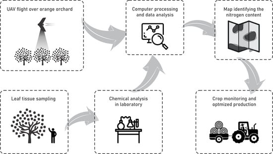
3. Materials and Method
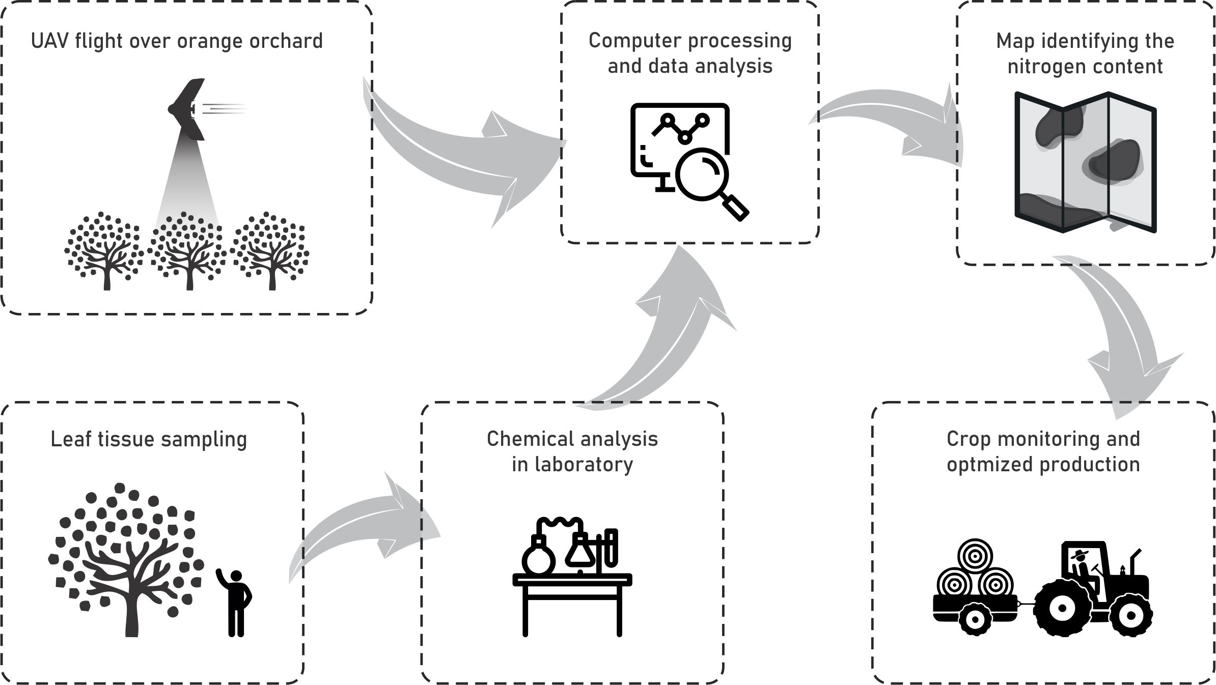
The proposed method consisted of three phases (Figure 1). Phase 1 describes the survey method performed to collect field data from a Valencia-orange orchard. Here we acquired aerial images with a multispectral Parrot Sequoia camera embedded in a UAV platform and collected leaf samples in the experimental area. Phase 2 focuses on image processing procedures. They were conducted in commercial software named Pix4DMapper, and sampling points were created in a geographical information system (GIS) environment with the open-source software QGIS 3.4. Phase 3 was separated into two stages. Primarily, we selected the available spectral indices for the Parrot Sequoia bands and compared the CNC with them. After that, we used these spectral indices as input parameters for our RF approach and evaluated it with a cross-validation method.

3.1. Data Survey

The study was conducted in a commercial orchard of Valencia orange (Citrus sinensis Valencia) trees planted on a Citrumelo swingle rootstock. The trees had reached their maturation stages at the period of the survey, with 5 years from their initial planting. The survey was carried out on 22 March 2018, when the plants were in their vegetative phase. The experiment was conducted in an area of 71.4 ha divided into 24 field-plots containing 752 plants per hectare, at 7 m × 1.9 m spacing (Figure 2). The area was previously fertilized with 250 kg.ha−1 of saturated nitrogen in ammonium nitrate.
The flight was conducted between 13:00 and 14:00. (local time), at 120 m high, resulting in a 12.9 cm ground sample distance (GSD) image. An eBee SenseFly UAV equipped with the Parrot Sequoia camera was used. This camera records images in the following spectral regions: green (530–570 nm), red (640–680 nm), red-edge (730–740 nm), and near-infrared (770–810 nm). Before the flight, a calibration plaque unique for the Sequoia equipment was recorded with the Parrot Sequoia camera to normalize the local illumination. The main characteristics of the UAV-mounted sensor used are summarized in Table 1.
The study area was separated into 27 field-plants (Figure 2). In each field, we collected an n amount of leaves from n number of trees. Both numbers variated according to plant-field size and the number of trees per field. In total, approximately 4000 leaf samplings were gathered in this area. The method applied here followed standard recommended procedures. For each citrus-tree sampled, we collected the 3rd or 4th leaf of a fruit-branch, at a medium canopy height. The leaves were all visually health with no signs of diseases or damage. They were separated and identified in plastic bags and submitted to the laboratory analysis.
In the laboratory, leaf area (cm2) was measured for each sample using a digital analysis method [37]. Later, they were washed and dried in an oven at 60–65 °C for 48 h, and then crushed. The Kjeldahl titration method was applied to determine the LNC. This method is divided into three stages: (1) digestion, (2) distillation in a nitrogen distiller, and (3) titration with sulfuric acid (H2SO4) [38]. After this, the averaged LNC values were associated with their correspondent field-plant. In our studied area, we obtained LNC between 23.2 and 29.5 g·kg−1, with a variance of 2.33 g·kg−1.

3.2. Image Pre-Processing and Sampling Points

The image pre-processing was performed in the Pix4DMapper software, in which we divided two mosaic blocks to optimize it (Figure 2). We first optimized the interior and exterior parameters and generated the sparse dense cloud based on the structure-from-motion (SfM) method. Later, we generated the point clouds based on MVS (multi-view stereo) approach. For the SfM, we used a total of nine control points in cross-format with approximately 50 cm × 50 cm in size, distributed equally in the experimental area. We measured the coordinates of these targets with a Leica Plus GS15 Global Navigation Satellite System (GNSS), dual-frequency in real-time kinematic (RTK) mode, with a 3 mm precision.
The UAV flight was approved by the Department of Airspace Control (DECEA), responsible for the Brazilian airspace. The images were acquired with an 80% longitudinal and 60% lateral overlaps. The orthomosaic was composed of 2389 scenes altogether. We converted the digital number (DN) values to surface reflectance values using the calibration parameters described in the Parrot Sequoia manual [39]. Finally, an orthorectified surface reflectance image was generated for each band at each block (I and II). Both image blocks were used to create a unique mosaic.
In a GIS environment, we manually identified 33,600 citrus-trees in our experimental area (Figure 2). This was performed in the QGIS 3.4 open-source software and used photointerpretation techniques to delineate point-features to mark the location of each tree. We attributed a radius (1.1–1.4 m) for each tree-canopy in order to calculate their respective leaf area index (LAI) in relation to the ground area. The mentioned variation in radius was used because of the difference in canopy sizes.
Light interaction at the canopy level is dominantly affected by canopy structure, and the leaf properties may be canceled out. Since our image data is at a landscape level, spectral vegetation indices should only be linked to LNC after considering this detail. To correctly compare average LNC measured in the laboratory with data extracted from the UAV-based image, we scaled up the LNC from leaf to canopy level (CNC). To do this, we multiplied the averaged LNC of each plant-field with the calculated LAI. This process can be described by Equation (1) [40]. This procedure resulted in 33,600 trees with known scaled up nitrogen content.
C N C = L N C l ¯   ×   L A I ,
where LNCl is the averaged value measured in the laboratory and LAI is given by the ratio between the leaf area and ground area. LNC was measured in g·kg−1, while LAI is dimensionless. The resulting CNC was also in g·kg−1. This equation is based on a canopy development model that considered the relationship between nitrogen content and the LAI at different growth stages [40,41]. In our study case, the citrus-trees were evaluated during their intermediate phase (i.e., with neither young or old leaves), so a linear relationship can be assumed [41].
We separated the trees into training and testing data-sets (Figure 2). The training points consisted of 90% (80% train and 10% validation) of the entire data-set, while the testing points were represented by the remaining 10%. We evaluated the distributions for the validation and testing data to determine if there was a significant difference between samples (Figure 3). This prior evaluation returned a normal distribution for both datasets (Shapiro–Wilk p-value equal to 0.77 and 0.79) and no statistical difference between both means (test t student p-value of 0.5144).

3.3. Spectral Vegetation Indices
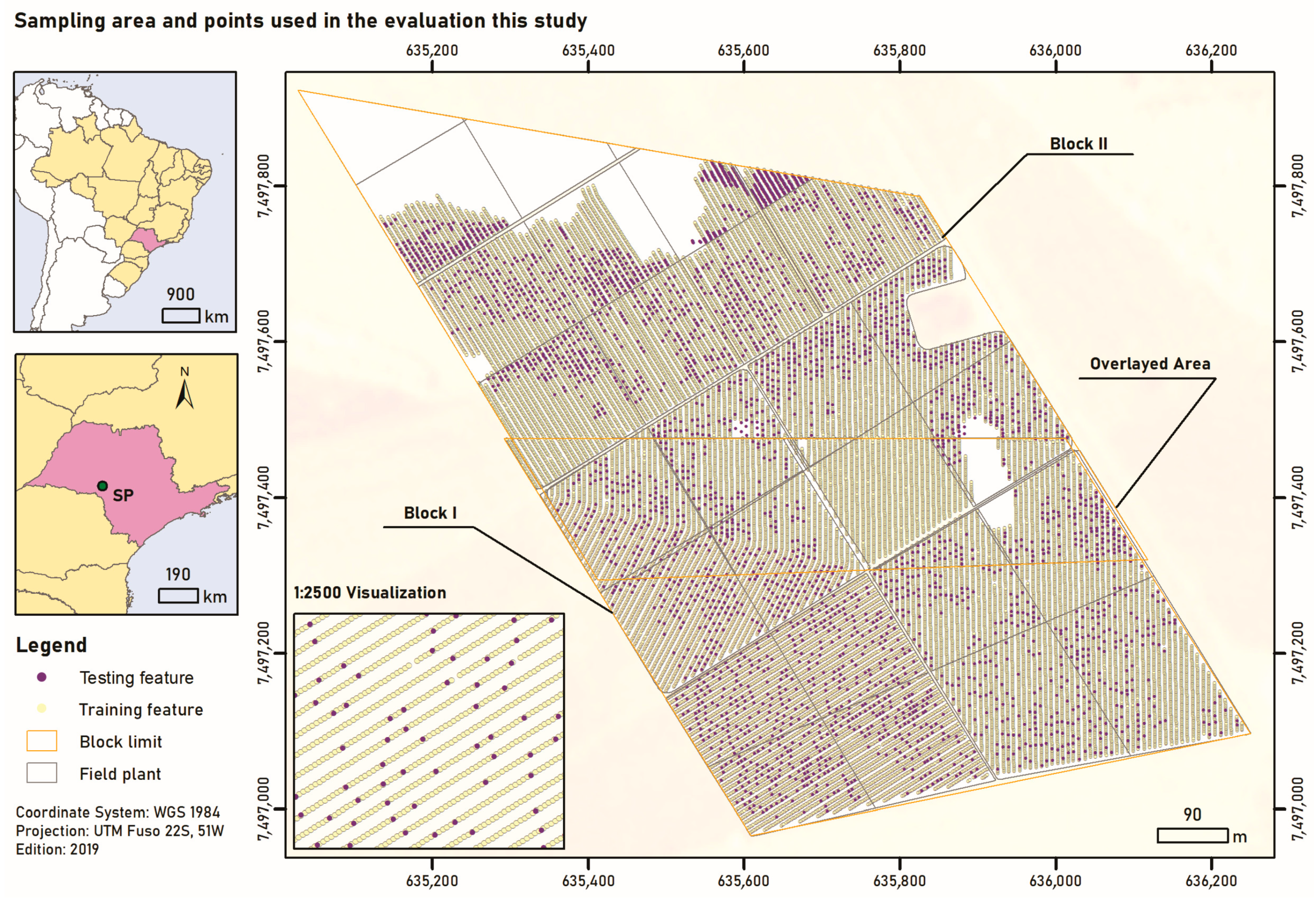
To gather the available spectral vegetation indices to this study, we based our selection on the Index Database [42]. We considered the spectral indices associates with the Parrot Sequoia band ranges (Table 2). We identified them according to their purpose (variable) and scale (canopy and/or leaf level). The values of parameters such as soil-lines (L), which are required by some spectral indices, were adopted based upon literature recommendation.
The relation between the spectral indices and the CNC was calculated using linear and exponential regressions. The metrics used to evaluate them were the regression coefficient (R2), the root-mean-squared error (RMSE), and the correlation coefficient (r) values. This prediction returned a statistical comparison for the individual spectral indices and helped evaluate their performance. For both regression and correlation analysis, we adopted a coefficient interval of 95%.

3.4. Analysis

The RF algorithm is based on regression trees and relies on the hypothesis that the overall accuracy can be improved by implementing the prediction results of combined independent predictors [20]. As previously stated, we distributed the 33,600 trees into training (80% train and 10% validation) and testing (10%) datasets. In a computational environment, we needed to define the number of trees, the number of nodes and the stop criteria for the RF model. To avoid overfitting, we performed a hyperparametrization process.
To define the most appropriate hyperparameter, we used a cross-validation stochastic approach, where we separated our dataset into 10 folds. One-fold was used to validate the model performance, while the remaining nine folds were used to train the model. This test was repeated until all the 10 folds were evaluated individually. In our study, the number of nodes did not interfere with the prediction accuracy, so a fixed parameter was adopted after initial tests. We determined the number of trees to be equal to 200 since it did not result in any practical gains with higher quantities (Figure 4).
We implemented an extreme gradient boosting (XGBoost) model to verify its impact on the RF performance. The XGBoost uses a forward-learning ensemble method to obtain predictive results in gradually improved estimations. This model computes second-order gradients of the loss function and an advanced regularization (L1 and L2) type [43]. We then performed an evaluation of the models’ accuracy when implementing less spectral indices. For this, we selected the 5 and 10 spectral indices that presented a higher contribution to our model. Lastly, since our RF model consisted of 200 trees, we evaluated its trees by a Pythagorean plot. As shorter trees are better in contributing to prediction values, we plotted one example of its first five levels to ascertain the relationship between the spectral indices in the RF model.
The compiled dataset was also used in other machine learning algorithms, like ANN, SVM, DT and LR [44]. These algorithms are considered standard approaches in machine learning evaluation and therefore were compared against RF to test its robustness. We applied the same conjunction of training and test data and performed their hyperparameterization. For this, we used a cross-validation stochastic approach, and data folds implemented in the RF evaluation were also used for these algorithms. The RF and the remaining machine learning algorithms were processed with the open-source RapidMiner 9.5 software, which runs in its own Python library [45]. The parameters of all methods have been set to the library default values except those described in this section.
The hyperparameterization process considered the individual characteristics of the evaluated algorithms. The stop criteria were defined once it did not reduce the MAE since it only increased the processing time needed. For the ANN algorithm, we adopted one hidden layer with 500 neurons and applied a linear activation function to the output layer. We also adopted the Adam Optimizer with a regularization (α) equal to 0.0001. The SVM was applied with a radial basis function (RBF) kernel exp(−g|x − y|2), where the gamma (g) value was set automatically, with a regression loss equal to 50.00, a tolerance of 0.001 and an interaction limit of 500. For the DT method, we determined the number of leaves to be equal or higher than 2 and adopted a maximum tree-depth of 100. Finally, we applied two regression models using the Ridge (L2) regularization and a Lasso (L1) regularization, with both strengths (α) equal to 0.015.
The proposed approach was evaluated with the following metrics: mean squared error (MSE); coefficient of variance of the root mean square error (CVRMSE); mean absolute error (MAE); and R2. We then qualitatively evaluated the RF predictions by plotting it in a regression graphic and also calculating the individual contribution of each spectral vegetation index for the model. Finally, we loaded the prediction results in a map, indicating the nitrogen content at each tree-canopy. For that, we created a new column feature in our tree dataset. This map was used to evaluate qualitatively the CNC through the experimental area.

4. Results

Spectral indices were computed to evaluate the direct relation with CNC in citrus-tress (Table 3). At least 12 of the tested spectral indices (total of 33) presented a regression coefficient above 0.5 and only 05 had a correlation coefficient higher than 0.7 in linear and exponential regressions. In literature, lower correlation values (0.5) have been used to determine regions favorable to the estimation of nitrogen content in citrus trees [31]. Though, in our study, most of these spectral indices presented RMSE higher than 1 g·kg−1, which is a considerable discrepancy for the CNC in our experimental area.
In our machine learning analysis, the proposed framework considering the RF model performed better than most of the other machine learning algorithms (Table 4) and individual spectral indices (Table 3). The algorithm returned a prediction with an MSE of 0.307 g·kg−1, and MAE of 0.341 g·kg−1 and an R2 equal to 0.90. The XGBoost model implemented also returned similar metrics.
Other algorithms like DT presented interesting results, being closer to the predictions of the RF model. This is to be expected since the random forest is based on the idea of multiple decision trees. Algorithms such as SVM, ANN, and LR had lower performances. However, they were still better than the previous individual spectral indices analysis.
The CNC predicted by the proposed framework with the RF was evaluated in a plot considering the measured CNC in comparison with the returned CNC from the prediction (Figure 5). Although the graphic shows some predictions distancing from the 1:1 relationship (dashed line), the high amount of data used (n = 3360) helped to estimate the result in a regression coefficient of 0.90. A slight decline in the line suggests that our approach was better at predicting CNC between 26 and 28 g·kg−1.
The contribution of each spectral index for the RF model (Figure 6) showed how the highest related spectral indices with CNC (Table 2) assisted the model into the prediction. This information should be considered when analyzing the performance of the model, since it may help future research to reduce the amount of data incorporated into the algorithm. For the prediction of CNC in citrus-trees, the returned results indicate a higher contribution of spectral vegetation indices like SR750–550 (8.2%), TriVI (7.3%), and CI (Red-edge; 6.2%). The first 10 spectral indices composed more than 55% of the contribution value (Figure 6).
By implementing the best five and 10 spectral indices into the RF model, we verified a slight decrease in its performance (Table 5). This is indicative of how even lower contributions may assist the model. Regardless, this decrease was relatively small, and a tradeoff between the number of spectral indices used and the obtained accuracy is something that should be considered. Another observation is that the XGBoost model presented better results, which may consist of an alternative to reduce the number of spectral indices while improving the performance of the algorithm.
A qualitative evaluation of one of the most representative trees returned by the random forest model helped ascertained the relationship between the spectral indices (Figure 7). An evaluation of shorter trees demonstrated that the best individual spectral indices (Figure 6) returned the strongest contributions.
The predictions returned by the proposed approach were incorporated into the map dataset. This procedure resulted in a qualitative map where a field technician can evaluate the CNC in each known citrus-tree with a prediction R2 of 0.90 (Figure 8).

5. Discussion

The proposed framework of this study predicted, with high accuracy (R2 of 0.90 and MSE of 0.307 g·kg−1), the amount of CNC present in citrus trees. In a previous study in the same area, we applied the SAM algorithm while submitting simulated spectral curves as input data, reaching an accuracy of 85.7% [36]. The method employed here allowed us to determine if machine learning models, specifically RF, were capable of performing this task. A contribution of this study is the use of spectral vegetation indices as input variables in a machine learning model to predict the amount of N2 at a tree-canopy level. The method presented here can be replicated to other orchards and cultivars once specifics such as sensor type and available spectral indices are considered.
As related, spectral indices have proved to be an important mechanism in the evaluation of N2 in other crops [22,23,24,25]. However, our results showed a low prediction accuracy (R2 below 0.7) by relating them directly to the CNC in the citrus-trees. Regardless, in the RF model, spectral indices developed considering red-edge bands generally performed better than other spectral indices. This observation was also found in the evaluation of the LNC in another study [33]. The majority of the high-relation indices also observed here were developed at the canopy level (Table 2).
The combination of spectral vegetation indices with machine learning models proved to be a suitable approach to predict CNC. The RF algorithm performed better than others, with decision tree being closely related. Other algorithms such as SVM and LRs showed similar accuracy to the individual spectral indices’ regression values. The ANN, although had a superior advantage over SVM and LRs, returned values far below the RF and DT algorithms. This comparison indicates how appropriate the regression analysis with RF is to predict CNC. This finding was also observed in other related studies [19,32,33,34].
The distribution of predicted values versus measured values (Figure 5) demonstrated how effective our approach was. Despite presenting errors in the extreme CNC ranges (23–24 and 29–30 g·kg−1), the model was able to reduce most errors in the intermediary values (26–28 g·kg−1). The high accuracy obtained can be explained because of the way the regression was calculated within the model since it considered the individual contribution of independent variables by combining its results. Still, it was recommended that future research always compare it against other machine learning algorithms.
We considered a total of 33 spectral indices, which was more than previous similar studies have used [19,33]. The individual contribution of each spectral index (Figure 6) demonstrated that the first 10 indices accounted for more than 55% of the total contribution for RF. Additionally, we performed evaluation tests considering the first five and 10 spectral indices (Table 5), in which also returned high accuracies. An evaluation of the shorter trees (Figure 7) corroborated the information shown by the individual spectral indices rank (Figure 6). Lastly, the XGBoost model helped to improve the accuracy of the algorithm when using a smaller number of spectral indices (Table 5). This indicates that it is possible to reduce the number of spectral indices used and still obtain highly accurate results. This information is important since it helps new researches to reduce the amount of processed data, which impacts training and testing time performances.
An adverse condition mentioned by other studies is the contribution of soil brightness to CNC evaluation. As spectral indices are directly obtained from reflectivity, it makes it difficult to avoid background effects [19]. However, in this study, since our data consisted only of delineated tree-canopies (Figure 2 and Figure 8), the soil-brightness contribution was considered minimal. Another possible impact is the anisotropy effect of the trees. Although spectral indices are known to reduce these effects, the fact that we scaled the leaf-measured LNC in the laboratory to an N2 in canopy-level should contribute to reducing this factor.
Finally, another contribution of our study was the construction of a map indicating the nitrogen content at a canopy level with an accurate prediction of 0.90 and an MSE of 0.307 g·kg−1. This type of map is effective as it may offer farmers and agronomic technicians the opportunity to evaluate individual plants. The agronomical method of collecting leaf-tissue and performing its chemical analysis in the laboratory is spatially limited due to practical reasons. Since our approach returned a high prediction for each individual tree, it is safe to assume that remotely sensed data outperforms the traditional method in relation to trees covered per area. This can positively impact fertilization methods and promote better yield predictions.

6. Conclusions

This study proposed a new framework to infer the nitrogen content at canopy-level in citrus trees. We evaluated the performance of the RF algorithm associated with spectral indices and compared it with other machine learning algorithms. Our approach demonstrated that the combination of spectral vegetation indices and the random forest algorithm is a powerful tool for CNC estimation. While a regression between the spectral indices and the CNC returned low coefficients (R2 at 0.10–0.63), the combined indices into the RF model resulted in an R2 of 0.90 and an MAE of 0.341 g·kg−1. This accuracy was higher than previous research, in which we evaluated spectral analysis algorithms for the same experimental field. In conclusion, we recommend the integration of spectral indices with machine learning algorithms like RF to assess CNC in citrus-trees.

Author Contributions

Conceptualization, L.P.O., A.P.M.R. and J.E.C.; methodology, L.P.O., É.A.S.M. and A.P.M.R.; formal analysis, L.P.O. and M.d.S.; resources, J.E.C., N.N.I., J.M.J. and E.T.M.; data curation, É.A.S.M. and L.P.O.; writing—original draft preparation, L.P.O. and A.P.M.R. writing—review and editing, J.M.J., D.R.P., J.L., V.L., W.N.G., N.E. and E.T.M.; supervision, A.P.M.R., J.M.J., N.N.I. and J.E.C.; project administration, L.P.O., A.P.M.R. and J.E.C.; funding acquisition, L.P.O. and J.E.C.

Funding

This research was partially funded by CAPES/Print (p: 88881.311850/2018-01). V. Liesenberg is supported by FAPESC (2017TR1762) and CNPq (313887/2018-7).

Conflicts of Interest

The authors declare no conflict of interest.

References

  1. Huang, S.; Miao, Y.; Yuan, F.; Cao, Q.; Ye, H.; Lenz-Wiedemann, V.I.S.; Bareth, G. In-season diagnosis of rice nitrogen status using proximal fluorescence canopy sensor at different growth stages. Remote Sens. 2019, 11, 1847. [Google Scholar] [CrossRef] [Green Version]
  2. Cui, B.; Zhao, Q.; Huang, W.; Song, X.; Ye, H.; Zhou, X. A new integrated vegetation index for the estimation of winter wheat leaf chlorophyll content. Remote Sens. 2019, 11, 974. [Google Scholar] [CrossRef] [Green Version]
  3. Zhang, K.; Ge, X.; Shen, P.; Li, W.; Liu, X.; Cao, Q.; Tian, Y. Predicting rice grain yield based on dynamic changes in vegetation indexes during early to mid-growth stages. Remote Sens. 2019, 11, 387. [Google Scholar] [CrossRef] [Green Version]
  4. Brinkhoff, J.; Dunn, B.W.; Robson, A.J.; Dunn, T.S.; Dehaan, R.L. Modeling mid-season rice nitrogen uptake using multispectral satellite data. Remote Sens. 2019, 11, 1837. [Google Scholar] [CrossRef] [Green Version]
  5. Tilly, N.; Bareth, G. Estimating nitrogen from structural crop traits at field scale—A novel approach versus spectral vegetation indices. Remote Sens. 2019, 11, 2066. [Google Scholar] [CrossRef] [Green Version]
  6. Li, Z.; Jin, X.; Yang, G.; Drummond, J.; Yang, H.; Clark, B.; Zhao, C. Remote sensing of leaf and canopy nitrogen status in winter wheat (Triticum aestivum L.) based on N-PROSAIL model. Remote Sens. 2018, 10, 1463. [Google Scholar] [CrossRef] [Green Version]
  7. Song, Y.; Wang, J. Soybean canopy nitrogen monitoring and prediction using ground based multispectral remote sensors. In Proceedings of the IEEE International Geoscience and Remote Sensing Symposium (IGARSS), Beijing, China, 10–15 July 2016; pp. 6389–6392. [Google Scholar] [CrossRef]
  8. Cilia, C.; Panigada, C.; Rossini, M.; Meroni, M.; Busetto, L.; Amaducci, S.; Boschetti, M.; Picchi, V.; Colombo, R. Nitrogen status assessment for variable rate fertilization in maize through hyperspectral imagery. Remote Sens. 2014, 6, 6549–6565. [Google Scholar] [CrossRef] [Green Version]
  9. Ciampitti, I.A.; Salvagiotti, F. New insights into soybean biological nitrogen fixation. Agron. J. 2018, 110, 1185–1196. [Google Scholar] [CrossRef] [Green Version]
  10. Chhabra, A.; Manjunath, K.R.; Panigraphy, S. Non-point source pollution in Indian agriculture: Estimation of nitrogen losses from rice crop using remote sensing and GIS. Int. J. Appl. Earth Obs. Geoinf. 2010, 12, 190–200. [Google Scholar] [CrossRef]
  11. Zheng, H.; Cheng, T.; Li, D.; Zhou, X.; Yao, X.; Tian, Y.; Zhu, Y. Evaluation of RGB, color-infrared and multispectral images acquired from unmanned aerial systems for the estimation of nitrogen accumulation in rice. Remote Sens. 2018, 10, 824. [Google Scholar] [CrossRef] [Green Version]
  12. Zheng, H.; Li, W.; Jiang, J.; Liu, Y.; Cheng, T.; Tian, Y.; Zhu, Y.; Cao, W.; Zhang, Y.; Yao, X. A Comparative assessment of different modeling algorithms for estimating LNC in winter wheat using multispectral images from an unmanned aerial vehicle. Remote Sens. 2018, 10, 2026. [Google Scholar] [CrossRef] [Green Version]
  13. Al-Najjar, H.A.H.; Kalantar, B.; Pradhan, B.; Saeidi, V.; Halin, A.A.; Ueda, N.; Mansor, S. Land cover classification from fused DSM and UAV images using convolutional neural networks. Remote Sens. 2019, 11, 1461. [Google Scholar] [CrossRef] [Green Version]
  14. Wu, L.; Zhu, X.; Lawes, R.; Dunkerley, D.; Zhang, H. Comparison of machine learning algorithms for classification of LiDAR points for characterization of canola canopy structure. Int. J. Remote Sens. 2019, 40, 5973–5991. [Google Scholar] [CrossRef]
  15. Dyson, J.; Mancini, A.; Frontoni, E.; Zingaretti, P. Deep learning for soil and crop segmentation from remotely sensed data. Remote Sens. 2019, 11, 1859. [Google Scholar] [CrossRef] [Green Version]
  16. Zhong, L.; Hu, L.; Zhou, H. Deep learning based multi-temporal crop classification. Remote Sens. Environ. 2019, 221, 430–443. [Google Scholar] [CrossRef]
  17. Wolanin, A.; Camps-Valls, G.; Gómez-Chova, L.; Mateo-García, G.; van der Tol, C.; Zhang, Y.; Guanter, L. Estimating crop primary productivity with Sentinel-2 and Landsat 8 using machine learning methods trained with radiative transfer simulations. Remote Sens. Environ. 2019, 225, 441–457. [Google Scholar] [CrossRef]
  18. Ashapure, A.; Oh, S.; Marconi, T.G.; Chang, A.; Jung, J.; Landivar, J.; Enciso, J. Unmanned aerial system based tomato yield estimation using machine learning. Proc. SPIE 11008, Autonomous Air and Ground Sensing Systems for Agricultural Optimization and Phenotyping IV. In Proceedings of the SPIE Defense + Commercial Sensing, Baltimore, MD, USA, 16–18 April 2019. [Google Scholar] [CrossRef]
  19. Pham, T.D.; Yokoya, N.; Bui, D.T.; Yoshino, K.; Friess, D.A. Remote sensing approaches for monitoring mangrove species, structure, and biomass: Opportunities and challenges. Remote Sens. 2019, 11, 230. [Google Scholar] [CrossRef] [Green Version]
  20. Liang, L.; Di, L.; Huang, T.; Wang, J.; Lin, L.; Wang, L.; Yang, M. Estimation of leaf nitrogen content in wheat using new hyperspectral indices and a random forest regression algorithm. Remote Sens. 2018, 10, 1940. [Google Scholar] [CrossRef] [Green Version]
  21. Krishna, G.; Sahoo, R.N.; Singh, P.; Bajpai, V.; Patra, H.; Kumar, S.; Sahoo, P.M. Comparison of various modelling approaches for water deficit stress monitoring in rice crop through hyperspectral remote sensing. Agric. Water Manag. 2019, 213, 231–244. [Google Scholar] [CrossRef]
  22. Shah, S.H.; Angel, Y.; Houborg, R.; Ali, S.; McCabe, M.F. A random forest machine learning approach for the retrieval of leaf chlorophyll content in wheat. Remote Sens. 2019, 11, 920. [Google Scholar] [CrossRef] [Green Version]
  23. Schlemmer, M.; Gitelson, A.; Schepers, J.; Ferguson, R.; Peng, Y.; Shanahan, J.; Rundquist, D. Remote estimation of nitrogen and chlorophyll contents in maize at leaf and canopy levels. Int. J. Appl. Earth Obs. Geoinf. 2013, 25, 47–54. [Google Scholar] [CrossRef] [Green Version]
  24. Huang, S.; Miao, Y.; Yuan, F.; Gnyp, M.L.; Yao, Y.; Cao, Q.; Wang, H.; Lenz-Wiedemann, V.I.S.; Bareth, G. Potential of RapidEye and WorldView-2 satellite data for improving rice nitrogen status monitoring at different growth stages. Remote Sens. 2017, 9, 227. [Google Scholar] [CrossRef] [Green Version]
  25. Kalacska, M.; Lalonde, M.; Moore, T.R. Estimation of foliar chlorophyll and nitrogen content in an ombrotrophic bog from hyperspectral data: Scaling from leaf to image. Remote Sens. Environ. 2015, 169, 270–279. [Google Scholar] [CrossRef]
  26. Chen, P.; Haboudane, D.; Tremblay, N.; Wang, J.; Vigneault, P.; Baoguo, L. New spectral indicator assessing the efficiency of crop nitrogen treatment in corn and wheat. Remote Sens. Environ. 2010, 114, 1987–1997. [Google Scholar] [CrossRef]
  27. Cammarano, D.; Fitzgerald, G.J.; Casa, R.; Basso, B. Assessing the robustness of vegetation indices to estimate wheat N in Mediterranean environments. Remote Sens. 2014, 6, 2827–2844. [Google Scholar] [CrossRef] [Green Version]
  28. Hunt, E.R.J.; Doraiswamy, P.C.; Mcmurtrey, J.E.; Daughtry, C.S.T.; Perry, E.M.; Akhmedov, B. A visible band index for remote sensing leaf chlorophyll content at the canopy scale. Int. J. Appl. Earth Obs. Geoinf. 2013, 21, 103–112. [Google Scholar] [CrossRef] [Green Version]
  29. Kooistra, L.; Clevers, J.G.P.W. Estimating potato leaf chlorophyll content using ratio vegetation indices. Remote Sens. Lett. 2016, 7, 611–620. [Google Scholar] [CrossRef] [Green Version]
  30. Zhai, Y.; Cui, L.; Zhou, X.; Gao, Y.; Fei, T.; Gao, W. Estimation of nitrogen, phosphorus, and potassium contents in the leaves of different plants using laboratory-based visible and near-infrared reflectance spectroscopy: Comparison of partial least-square regression and support vector machine regression methods. Int. J. Remote Sens. 2013, 34, 2502–2518. [Google Scholar] [CrossRef]
  31. Min, M.; Lee, W. Determination of significant wavelengths and prediction of nitrogen content for citrus. Am. Soc. Agric. Eng. 2005, 48, 455–461. [Google Scholar] [CrossRef]
  32. Xiong, X.; Zhang, J.; Guo, D.; Chang, L.; Huang, D. Non-Invasive Sensing of Nitrogen in Plant Using Digital Images and Machine Learning for Brassica Campestris ssp. Chinensis L. Sensors 2019, 19, 2448. [Google Scholar] [CrossRef] [Green Version]
  33. Abdel-Rahman, E.M.; Ahmed, F.B.; Ismail, R. Random forest regression and spectral band selection for estimating sugarcane leaf nitrogen concentration using EO-1 Hyperion hyperspectral data. Int. J. Remote Sens. 2013, 34, 712–728. [Google Scholar] [CrossRef]
  34. Ramoelo, A.; Cho, M.A.; Mathieu, R.; Madonsela, S.; van de Kerchove, R.; Kaszta, Z.; Wolff, E. Monitoring grass nutrients and biomass as indicators of rangeland quality and quantity using random forest modelling and WorldView-2 data. Int. J. Appl. Earth Obs. Geoinf. 2015, 43, 43–54. [Google Scholar] [CrossRef]
  35. Liu, X.F.; Lyu, Q.; He, S.L.; Yi, S.L.; Hu, D.Y.; Wang, Z.T.; Deng, L. Estimation of carbon and nitrogen contents in citrus canopy by low-altitude remote sensing. Int. J. Agric. Biol. Eng. 2016, 9, 149–157. [Google Scholar] [CrossRef]
  36. Osco, L.P.; Marques Ramos, A.P.; Saito Moriya, É.A.; de Souza, M.; Marcato Junior, J.; Matsubara, E.T.; Creste, J.E. Improvement of leaf nitrogen content inference in Valencia-orange trees applying spectral analysis algorithms in UAV mounted-sensor images. Int. J. Appl. Earth Obs. Geoinf. 2019, 83, 101907. [Google Scholar] [CrossRef]
  37. Katabuchi, M. LeafArea: An R package for rapid digital image analysis of leaf area. Ecol. Res. 2015, 30, 1073–1077. [Google Scholar] [CrossRef]
  38. Nitrogen Determination by Kjeldahl Method PanReac AppliChem ITW Reagents. Available online: https://www.itwreagents.com/uploads/20180114/A173_EN.pdf (accessed on 9 February 2019).
  39. Sequoia, P. Parrot Sequoia Manual. © 2019 Parrot Drones SAS. Available online: https://parrotcontact.parrot.com/website/user-guides/sequoia/sequoia_user_guide.pdf (accessed on 19 November 2019).
  40. Ling, B.; Goodin, D.G.; Mohler, R.L.; Laws, A.N.; Joern, A. Estimating canopy nitrogen content in a heterogeneous grassland with varying fire and grazing treatments: Konza Prairie, Kansas, USA. Remote Sens. 2014, 6, 4430–4453. [Google Scholar] [CrossRef] [Green Version]
  41. Yin, X.; Lantinga, E.A.; Schapendonk, A.H.C.M.; Zhong, X. Some quantitative relationships between leaf area index and canopy nitrogen content and distribution. Ann. Bot. 2003, 91, 893–903. [Google Scholar] [CrossRef] [Green Version]
  42. IDB. Index DataBase. A Database for Remote Sensing Indices. The IDB Project, 2011–2019. Available online: https://www.indexdatabase.de/ (accessed on 7 February 2019).
  43. XGBoost. eXtreme Gradient Boosting. Available online: https://github.com/dmlc/xgboost (accessed on 23 November 2019).
  44. Mitchell, T.M. Machine Learning, 1st ed.; McGraw-Hill, Inc.: New York, NY, USA, 1997. [Google Scholar]
  45. RapidMiner. RapidMiner Python Package. Available online: https://github.com/rapidminer/python-rapidminer (accessed on 23 November 2019).
Figure 1. The workflow of the steps of the proposed method.
Remotesensing 11 02925 g001
Figure 2. Study area and points used in the evaluation of the spectral indices.
Remotesensing 11 02925 g002
Figure 3. Distribution of spectral sampling points as a function of leaf nitrogen content (LNC).
Remotesensing 11 02925 g003
Figure 4. Training accuracy with the difference in accuracy for the random forest (RF) model.
Remotesensing 11 02925 g004
Figure 5. Random forest model prediction for the CNC in citrus (23–30 g·kg−1).
Remotesensing 11 02925 g005
Figure 6. Individual contribution (in %) of each spectral vegetation index for the RF model.
Remotesensing 11 02925 g006
Figure 7. Example of one short tree (initial 5-levels) of the RF model applied.
Remotesensing 11 02925 g007
Figure 8. High-detailed image example of the CNC predicted with the RF model loaded in the entire dataset.
Remotesensing 11 02925 g008
Table 1. Parrot Sequoia camera details and flight conditions.
BandWavelength (nm)Spectral Resolution10 BitsFlight High120 m
Green550 (± 40)Spatial Resolution12.9 cmFlight Time01:30 P.M.
Red660 (± 40)HFOV70.6°WeatherPartially cloudy
Red-edge735 (± 10)VFOV52.6°Precipitation0 mm
Near-infrared790 (± 40)DFOC89.6°WindAt 1–2 m/s
Horizontal field of view (HFOV); vertical field of view (VFOV); displayed field of view (DFOC).
Table 2. The spectral vegetation indices associated with the Sequoia camera used in this study.
IndexEquationVariableScale
ARVI2 (Atmospherically Resistant Vegetation Index 2) 0.18 + 1.17 [ ( R λ nir   R λ red ) ( R λ nir +   R λ red ) ] VitalityCanopy
CCCI (Canopy Chlorophyll Content Index) ( R λ nir   R λ rededge ) / ( R λ nir +   R λ rededge ) ( R λ nir   R λ red ) / ( R λ nir +   R λ red ) ChlorophyllLeaf/Canopy
CG (Chlorophyll Green) ( R λ nir / R λ green ) 1 ChlorophyllLeaf/Canopy
CIgreen (Chlorophyll Index Green) ( R λ nir / R λ green ) 1 Chlorophyll/LAILeaf/Canopy
CIrededge (Chlorophyll Index RedEdge) ( R λ nir / R λ rededge ) 1 Chlorophyll/LAILeaf/Canopy
Ctr2 (Simple Ratio 695/760 Carter2) R λ rededge / R λ nir Chlorophyll/StressLeaf
CTVI (Corrected Transformed Vegetation Index) NDVI + 0.5 | NDVI + 0.5 | NDVI + 0.5 VegetationLeaf/Canopy
CVI (Chlorophyll Vegetation Index) R λ nir ( R λ red / R λ green 2 ) ChlorophyllCanopy
GDVI (Difference NIR/Green Difference Vegetation Index) R λ nir   R λ green VegetationLeaf
GI (Simple Ratio 554/677 Greenness Index) R λ green / R λ red ChlorophyllLeaf
GNDVI (Normalized Difference NIR/Green NDVI) ( R λ nir   R λ green ) / ( R λ nir +   R λ green ) ChlorophyllLeaf
GRNDVI (Green-Red NDVI) R λ nir ( R λ green +   R λ red ) R λ nir +   ( R λ green +   R λ red ) VegetationLeaf/Canopy
GSAVI (Green Soil Adjusted Vegetation Index) ( 1 + L ) ( R λ nir   R λ green ) ( R λ nir +   R λ green + L ) VegetationCanopy
IPVI (Infrared Percentage Vegetation Index) R λ nir ( R λ nir +   R λ red 2 ) ( NDVI + 1 ) VegetationCanopy
MCARI1 (Modified Chlorophyll Absorption in Reflectance Index 1) 1.2 [ 2.5 ( R λ nir R λ red ) 1.3 ( R λ nir   R λ green ) ] ChlorophyllLeaf/Canopy
MSAVI (Modified Soil Adjusted Vegetation Index) [ 2 R λ nir + 1 ( 2 R λ nir + 1 ) 2 8 ( R λ nir   R λ red ) ] 2 VegetationCanopy
MSR (Modified Simple Ratio) ( SR 1 ) / ( SR + 1 ) VegetationLeaf
MTVI (Modified Triangular Vegetation Index) 1.2 [ 1.2 ( R λ nir R λ green ) 2.5 ( R λ red   R λ green ) ] VegetationLeaf/Canopy
ND682/553 (Normalized Difference 682/553) ( R λ red   R λ green ) / ( R λ red +   R λ green ) VegetationLeaf/Canopy
NDVI (Normalized Difference Vegetation Index) ( R λ nir   R λ red ) / ( R λ nir +   R λ red ) Biomass/OthersLeaf/Canopy
Norm G (Normalized G) R λ green / ( R λ nir + R λ red + R λ green ) VegetationLeaf/Canopy
Norm NIR (Normalized NIR) R λ nir / ( R λ nir + R λ red + R λ green ) VegetationLeaf/Canopy
Norm R (Normalized R) R λ red / ( R λ nir + R λ red + R λ green ) VegetationLeaf/Canopy
OSAVI (Optimized Soil Adjusted Vegetation Index)I ( 1 + 0.16 ) ( R λ nir   R λ red ) ( R λ nir +   R λ red + 0.16 ) VegetationCanopy
RDVI (Renormalized Difference Vegetation Index) ( R λ nir   R λ red ) / ( R λ nir +   R λ red ) ChlorophyllLeaf/Canopy
SAVI (Soil-Adjusted Vegetation Index)II ( 1 + L ) ( R λ nir   R λ red ) ( R λ nir +   R λ red + L ) BiomassCanopy
SR672/550 (Simple Ratio 672/550 Datt5) R λ red / R λ green ChlorophyllLeaf
SR750/550 (Simple Ratio 750/550 Gitelson and Merzlyak 1) R λ rededge / R λ green ChlorophyllLeaf/Canopy
SR800/550 (Simple Ratio 800/550) R λ nir / R λ green Chlorophyll/BiomassLeaf
TraVI (Transformed Vegetation Index) NDVI + 0.5 VegetationLeaf/Canopy
TriVI (Triangular Vegetation Index) 0.5 [ 120 ( R λ rededge R λ green ) 200 ( R λ red   R λ green ) ] ChlorophyllLeaf/Canopy
SR (Simple Ratio) R λ nir / R λ red VegetationLeaf
WDRVI (Wide Dynamic Range Vegetation Index) ( 0.1 R λ nir   R λ red ) / ( 0.1 R λ nir +   R λ red ) Biomass/LAILeaf/Canopy
L = 0.5; NDVI = normalized differential vegetation index; SR = simple ratio; LAI = leaf area index. The variable “Vegetation” indicates that the applicability of the index occurs in a general sense, and is not specific like the others; NIR = near-infrared. Central wavelengths are indicated in Table 1.
Table 3. Regression analysis between the spectral vegetation indices and the canopy nitrogen content (CNC).
IndexR2RMSEEquationr
ARVI20.122.014y = 67.36x − 31.180.3504
CCCI0.571.145y = 86.55x − 0.0041210.6954
CG0.571.123y = 3.008x − 5.7820.6796
CIgreen0.261.853y = 3.008x − 2.7740.4796
CIrededge0.571.223y = 26.13x + 6.7140.6072
Ctr20.112.031y = −125.5x + 34.09−0.2282
CTVI0.122.020y = 178.9x − 184.10.2430
CVI0.511.359y = 3.572x + 0.21910.6424
GDVI0.431.515y = −698.6x2 + 607.1x − 104.90.5996
GI0.301.797y = −23.09x + 62.69−0.3493
GNDVI0.421.431y = 186x − 126.60.5853
GRNDVI0.261.821y = 82.78x − 33.620.3996
GSAVI0.521.279y = −1608x2 + 1989x − 588.10.6690
IPVI0.132.006y = 87.83x − 51.580.2607
MCARI10.451.188y = −394.2x2 + 523.7x − 46.90.5731
MSAVI0.621.013y = −1748x2 + 2431x − 817.10.7626
MSR0.231.887y = 6.52x + 2.1010.3792
MTVI0.451.288y = −394.2x2 + 523.7x − 46.90.5731
ND682/5530.112.029y = 37x + 33.790.2319
NDVI0.122.014y = 78.81x − 43.30.2504
Norm G0.471.134y = −438.4x + 63.11−0.6188
Norm NIR0.321.621y = 165.6x − 116.40.4996
Norm R0.112.030y = −168.6x + 35.29−0.2288
OSAVI0.391.529y = 68.43x − 25.890.5032
RDVI0.541.154y = −2168x2 + 2671x − 795.30.6028
SAVI0.581.045y = −2123x2 + 2747x − 861.50.6813
SR672/5500.102.175y = −881.4x2 + 1197x − 379.40.0982
SR750/5500.611.022y = 7.301x − 18.770.7991
SR800/5500.571.083y = 3.008x − 5.7820.7296
TraVI0.122.020y = 178.9x − 184.10.2430
TriVI0.631.001y = −0.782x2 + 24.49x − 164.30.8012
VIN0.271.832y = 0.9866x + 9.7540.3238
WDRVI0.581.076y = −466.2x2 + 238.9x − 3.6660.7166
Indices highlighted showed a regression coefficient (R2) above 0.50. All spectral indices returned a p-value under 0.05.
Table 4. Performance results of each selected algorithm prediction evaluated in this study.
ModelMSECVRMSEMAER2
Support Vector Machine2.0555.1491.0110.65
Decision Tree0.3472.2250.4620.85
Random Forest0.3072.0980.3410.90
Random Forest (XGBoost)0.3002.0430.3270.90
Artificial Neural Network1.6764.1680.8650.70
Linear Regression (Ridge)2.0415.8950.9840.63
Linear Regression (Lasso)2.0105.7900.9650.65
Table 5. Performance results of the random forest model with less spectral indices as input.
ModelIndices (n)MSECVRMSEMAER2
Random Forest50.3762.3420.4770.83
Random Forest (XGBoost)50.3502.2530.4120.85
Random Forest100.3452.2150.4010.85
Random Forest (XGBoost)100.3182.1270.3570.88

